1. Introduction
Pipelines serve as vital conduits in both industrial and daily life, bearing critical responsibilities,such as energy transmission, water resource distribution, and industrial fluid conveyance. Their safe operation is intrinsically linked to national security and protection of citizens' lives and property.Owing to the environmental conditions and operational lifespan, pipelines are susceptible to defects such as corrosion, deformation, and fractures, which compromise their service life and pose significant safety hazards. Statistics indicate that in the United States, pipeline defects result in annual economic losses exceeding
$130 billion. As a major industrial power, China employs pipelines extensively; annually, direct economic damages caused by pipeline-related accidents due to defects reach over
$200 billion [
1]. Consequently, the development of efficient and high-precision defect detection methods plays a crucial role in preventing and mitigating pipeline failure disasters. Traditional detection approaches, such as manual inspection, rely heavily on human judgment, which introduces subjectivity and increases the likelihood of missed or false detections. These methods are often constrained by environmental factors, leading to low inspection efficiency and poor adaptability to extreme conditions. As a result, manual inspection techniques are increasingly inadequate to meet the demands of modern industrial production.
In addition, mainstream nondestructive testing methods such as ultrasonic testing, magnetic flux leakage testing, and eddy current testing have been widely applied for defect detection since the last century [
2]. Although these techniques significantly improve detection accuracy and efficiency compared to manual inspection, they are heavily constrained by the material properties of the tested objects, resulting in limited versatility and unsuitability for pipelines made of materials other than metals. Some methods are also operationally complex; for example, magnetic flux leakage testing requires magnetizing the object beforehand, which is time-consuming and labor-intensive. Nowadays, pipeline materials have diversified in response to industrial production demands, including but not limited to concrete, plastic pipes (PVC), and fiberglass-reinforced plastic (FRP). These materials are incompatible with the aforementioned detection techniques.
In recent years, with the continuous development of deep learning and machine vision, it has gradually become the mainstream method in pipeline defect detection due to its advantages of non-contact detection, fast response speed and high detection accuracy.Object detection algorithms are primarily categorized into two-stage detection algorithms and single-stage detection algorithms [
3].The two-stage detection algorithms are exemplified by Faster R-CNN, which employs a core methodology of generating candidate regions via a Region Proposal Network (RPN), followed by classification and regression of these regions [
4]. This sequential processing mechanism effectively enhances detection accuracy. In contrast, single-stage detection algorithms [
5], represented by the YOLO series and SSD, utilize an end-to-end detection approach that performs dense predictions directly on feature maps, eliminating the candidate region generation step. This design significantly accelerates detection speed while maintaining a high level of precision.
Compared to two-stage detection algorithms, the YOLO series is highly regarded in the field of object detection due to its numerous advantages, including low computational overhead, rapid processing speed, real-time performance, streamlined algorithm implementation, and simplified training and deployment processes. These attributes enable it to effectively meet the demands of modern industrial production. In recent years, there has been sustained experimental interest in optimizing and improving the YOLO model.JiangChao Z et al. [
6] enhanced the YOLOv5 algorithm by integrating the Enhanced Convolutional Block Attention Module (ECBAM) and the Switchable Atrous Convolution (SAC) modules, effectively strengthening the model's focus on key features while suppressing irrelevant information. Additionally, the adoption of the SIOU loss function provided a more comprehensive assessment of the alignment between predicted and ground truth bounding boxes. These improvements collectively led to significant performance enhancements across various metrics in pipeline defect detection tasks.Wang T. et al. [
7] proposed an improved model based on YOLOv5s, incorporating the Squeeze-and-Excitation (SE) module and GSConv structures within the backbone and feature fusion networks to enhance detection accuracy and streamline the model architecture. Additionally, the integration of the CBAM attention mechanism bolstered the model's ability to recognize objects in complex backgrounds. The application of knowledge distillation further elevated the model's performance, effectively addressing the issues of subjectivity, low efficiency, and deployment challenges in CCTV pipeline defect detection.Zhao X et al. [
8] proposed an improved algorithm model, CEM-YOLO, based on YOLOv7. This model integrates the CARAFE sampling strategy, which maintains feature extraction capabilities while effectively reducing computational costs and accelerating detection speed. Additionally, an Enhanced Variance-Center Feature Pyramid (EVC) module was introduced, significantly enhancing the model's ability to detect and recognize small-scale targets.Finally, the MPDIoU loss function was replaced to expedite model convergence and improve localization accuracy.Wu Zhehaoet al. [
9] proposed an improved drainage pipe defect detection model based on EfficientViT integrated with YOLOv8. The model replaces the backbone network of YOLOv8 with an EfficientViT feature extraction network, effectively reducing the number of parameters. Subsequently, the SE attention mechanism is introduced to enhance the model's ability to capture key features, thereby improving robustness. Finally, Focal Loss is employed to mitigate the impact of easy negative samples, resulting in a more stable convergence of the optimized model.
Although the aforementioned model optimization methods each offer distinct advantages in enhancing detection accuracy, simplifying model architecture, and strengthening feature extraction capabilities, they inevitably introduce issues such as increased model parameter counts, higher computational costs, and diminished robustness. These limitations make them ill-suited for meeting the resource-constrained and real-time demands of current industrial production environments. Therefore, this paper proposes a lightweight pipeline defect detection algorithm based on FALW-YOLOv8. This algorithm introduces FasterBlock into the C2f module of the YOLOv8 baseline model's Backbone and Neck, accelerating feature propagation while conserving computational resources. It replaces traditional downsampling convolutions with ADown downsampling to mitigate feature loss in small objects. Additionally, the LSKA attention mechanism is incorporated into the Neck to suppress complex background interference, further enhancing the model's feature response capability. Finally, the Wise-IoU v2 loss function optimizes regression accuracy for difficult samples, accelerates model convergence, and enhances robustness.
2. Pipeline Defect Detection Algorithm
2.1. YOLOv8 Baseline Model
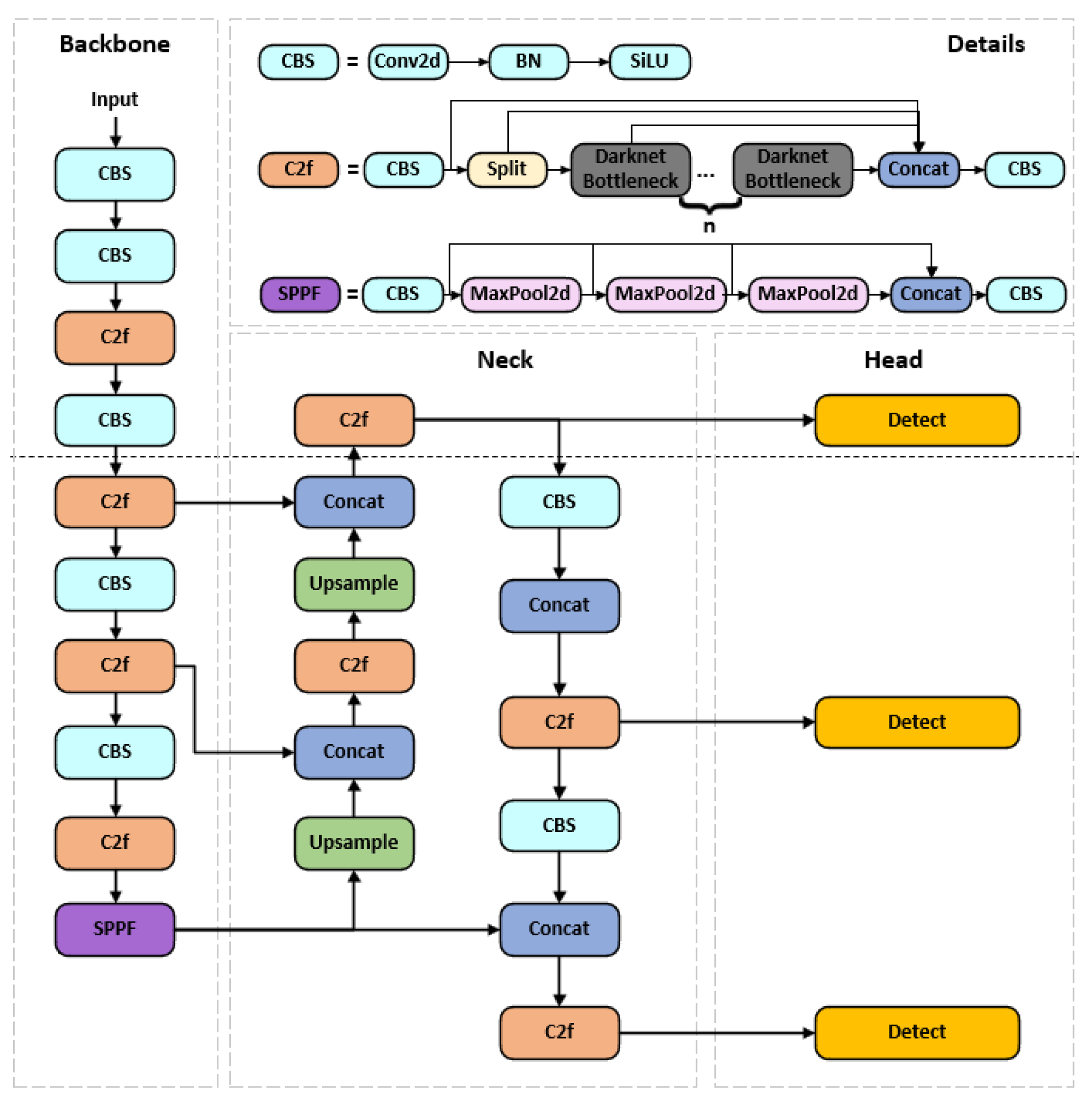
The YOLOv8 baseline model primarily consists of three components: the Backbone, Neck, and Head. Its network architecture is illustrated in
Figure 1.
The backbone network serves as the foundation of the entire model, undertaking the critical task of extracting multilevel features from raw images. This network comprises the CBS module, C2f module, and SPPF module. The CBS module acts as the fundamental building block, achieving normalized feature extraction through a combination of convolutional layers (Conv), batch normalization (BN), and the SILU activation function. The cross-stage partial connection design in the C2f module significantly enhances gradient flow and feature reuse efficiency by splitting feature maps, processing them through Bottleneck residual blocks, and then reassembling them. The SPPF module employs a serial max-pooling strategy to capture multi-scale information, improving computational efficiency.
The Neck Network serves as the feature fusion layer, employing a PAN-FPN architecture. Through a bidirectional feature pyramid design, it achieves multi-level feature fusion, optimizing multi-scale object detection capabilities.
The Detection Head incorporates three scales—large, medium, and small—to perform final predictions on the multi-scale features extracted earlier, including bounding box regression, category information, and confidence scores. Furthermore, its Anchor-Free design simplifies the training process and enhances flexibility, while its decoupled head structure effectively reduces task conflicts, thereby improving the model's overall performance.
2.2. FALW-YOLOv8 Enhanced Model
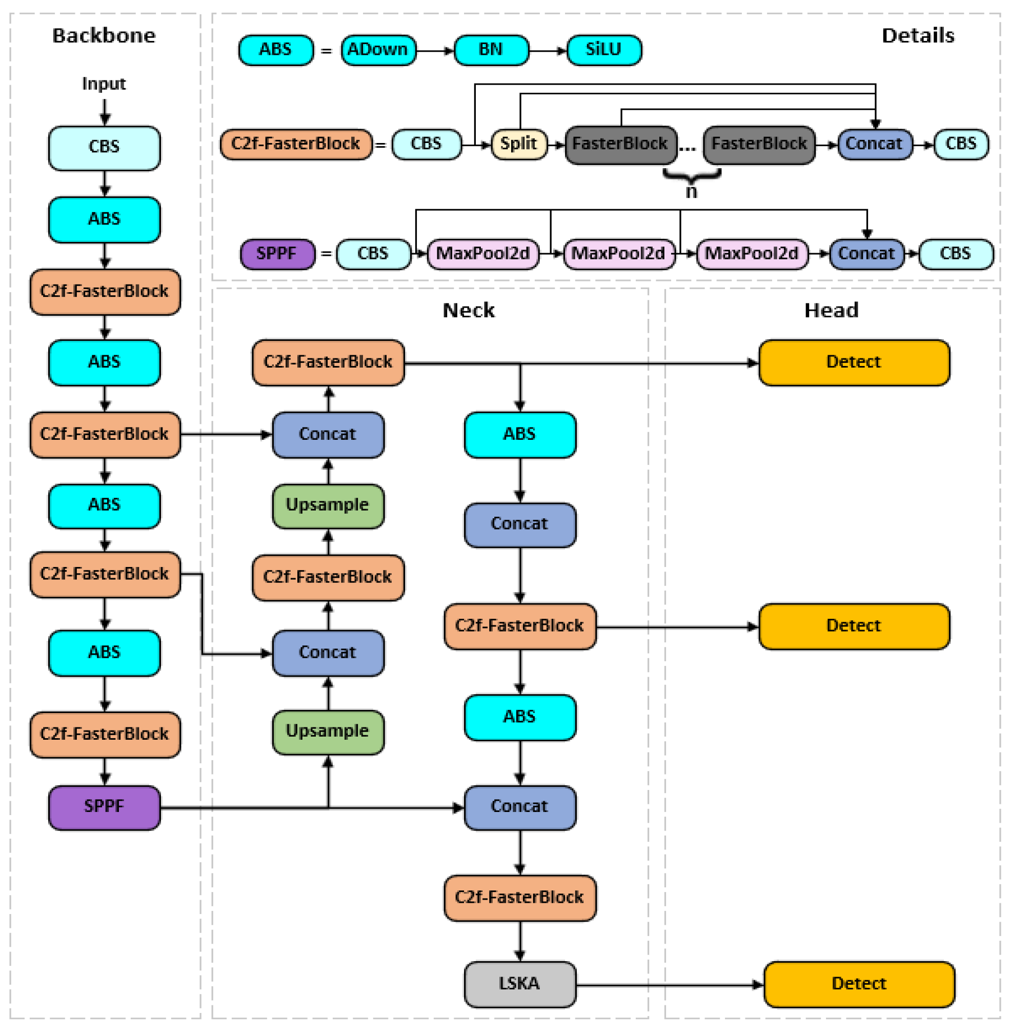
Although the YOLOv8 baseline model demonstrates strong performance in both detection speed and accuracy, it still suffers from limitations such as inadequate detection of small objects, poor adaptability to complex backgrounds, and high computational costs due to its large parameter count. These shortcomings make it difficult to meet the demands of pipeline defect detection tasks, which involve complex detection environments, high real-time requirements, and limited computational resources. Therefore, this paper proposes the following improvements to the YOLOv8 baseline model. The network architecture diagram of the improved FALW-YOLOv8 model is shown in
Figure 2.
2.2.1. FasterBlock Module
As the core submodule of FasterNet [
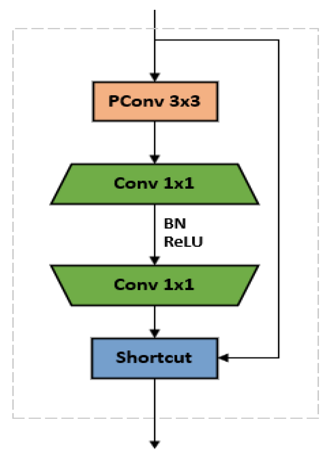
10], FasterBlock is a lightweight feature extraction module optimized for real-time object detection. Its internal structure is illustrated in
Figure 3.
As shown in the structural diagram, the input feature map first enters the partial convolution layer. After completing the convolution operation on partial channels, it sequentially passes through two pointwise convolution layers to perform channel expansion and channel compression, forming an inverted residual structure. During this process, each pointwise convolution layer is followed by a BN layer and a ReLU activation function to accelerate training and introduce nonlinear transformations. Finally, the original input feature map is directly added to the feature map processed by partial convolution and pointwise convolution through residual connections. This completes the feature information fusion before outputting the final feature map.
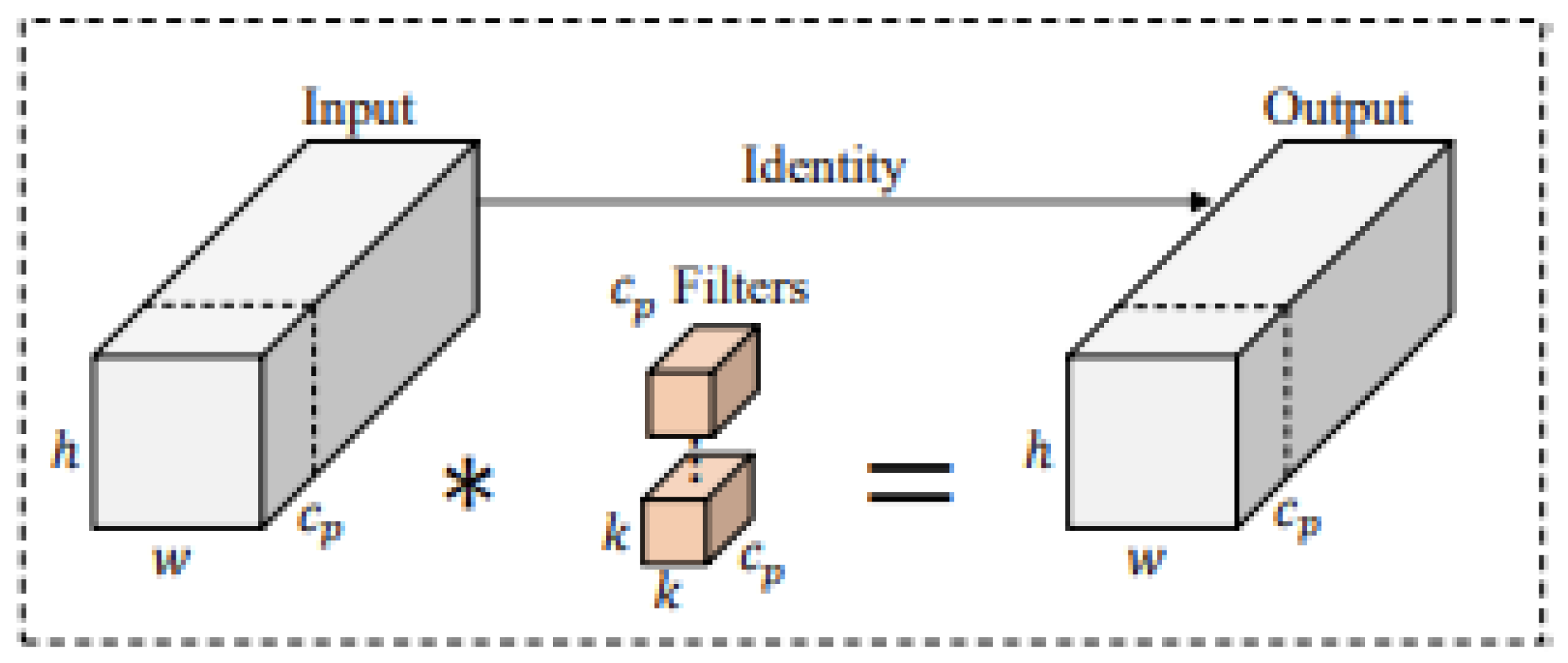
Partial Convolution Layer (PConv) is a core component of the FasterBlock module. Its fundamental principle leverages feature redundancy—where multiple channels of the input feature map often contain similar information such as edges and textures, leading to significant computational duplication. PConv performs spatial feature extraction only on a subset of channels (typically half the total number), while preserving the original features in the remaining channels. The structural diagram is shown in
Figure 4.
According to the structural diagram, assume that the input feature map,In the formula:represents the number of input channels;represents the spatial dimensions.
Set the channel grouping count to(typically set to 4),PConv then performs convolution processing onchannels:;In the formula, denotes a 3x3 convolution operation;Indicates the feature maps of the firstchannels.From the above operations, it can be seen that the computational complexity of PConv is:(3×3 core);Compared to conventional convolutions:(3×3 core);When the channel grouping count is set to 4,PConv reduces computational complexity to one-sixteenth that of classical convolutions, significantly lowering computational overhead and accelerating model inference speed.
The feature information processed through convolution is fed into the Pointwise Convolution layer (PWConv), where 1x1 convolutions perform feature transformation and information aggregation along the channel dimension. This layer can be divided into two steps: channel expansion and channel compression:
Channel Extension: Map the number of input channels fromto(is the expansion ratio) to enhance feature expression capabilities.
Channel Compression:Map the number of channels from back to the original dimension , ensuring consistent feature map
dimensions and restoring the channel dimension to reduce computational burden
on subsequent layers.
Pointwise Convolution essentially achieves efficient transformation and fusion across channel dimensions at minimal computational cost. It effectively addresses the lack of interaction between channels in deep convolutions, resolving the inability to fuse cross-channel correlations. PWConv reconstructs the channel dimension, linearly combining features from different channels with nonlinear activation to form a joint cross-channel representation, thereby enabling parameter sharing across spatial dimensions.
Finally, the residual connection adds the input feature map x to the output F(x) of the MLP layer to obtain the final output:
;In this formula,
represents a variant of Dropout [
11] that randomly disconnects residual paths to prevent overfitting while enhancing feature reuse and improving model stability. The residual connection module employs direct gradient transmission via an identity mapping, enabling gradients to propagate directly from the output layer back to the input layer during backpropagation. This effectively avoids the gradient decay caused by chain rule multiplication in traditional methods.The gradient of the loss function L with respect to the input x can be expressed as follows:
;In the equation,
represents the identity matrix (the gradient of the identity mapping), which ensures that the underlying gradient preserves at least the original signal, thereby preventing the vanishing gradient problem caused by excessively small values of
.
2.2.2. ADown Module
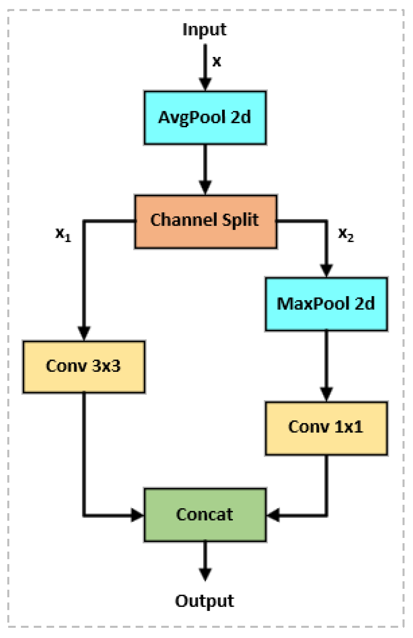
As a lightweight adaptive downsampling module, ADown reduces the spatial resolution of feature maps by dynamically adjusting its downsampling strategy, while incorporating multi-scale feature fusion and lightweight techniques to preserve more semantic information such as edges and textures [
12]. Its internal structure is illustrated in
Figure 5.
As shown in the block diagram, when ADown performs downsampling, the input feature map first passes through an average pooling layer [
13]. This layer performs preliminary downsampling on the feature map, reducing its spatial resolution while preserving smoother feature distributions and minimizing information loss. Subsequently, the mean-pooled feature map is split into two parts along the channel dimension. One part undergoes a 3x3 convolution operation to further reduce the spatial dimension and extract information features. The other part first undergoes max pooling, followed by a 1x1 convolution layer to adjust its channel count and introduce nonlinearity. Finally, the feature information processed through these two paths is fused and concatenated along the channel dimension to obtain the final output feature map.
The ADown subsampling module addresses issues inherent in traditional subsampling, such as inability to adapt to targets of varying scales or types, severe information loss, and low computational efficiency caused by conventional max pooling and fixed stride convolutions. It achieves this by splitting the input feature map into multiple branches, applying distinct subsampling strategies to each branch, and finally fusing the results. Simultaneously, it dynamically adjusts kernel size, stride, or fusion weights based on input feature information. This approach preserves more semantic information and enhances the model's feature representation capabilities.
2.2.3. LSKAttention Attention Mechanism
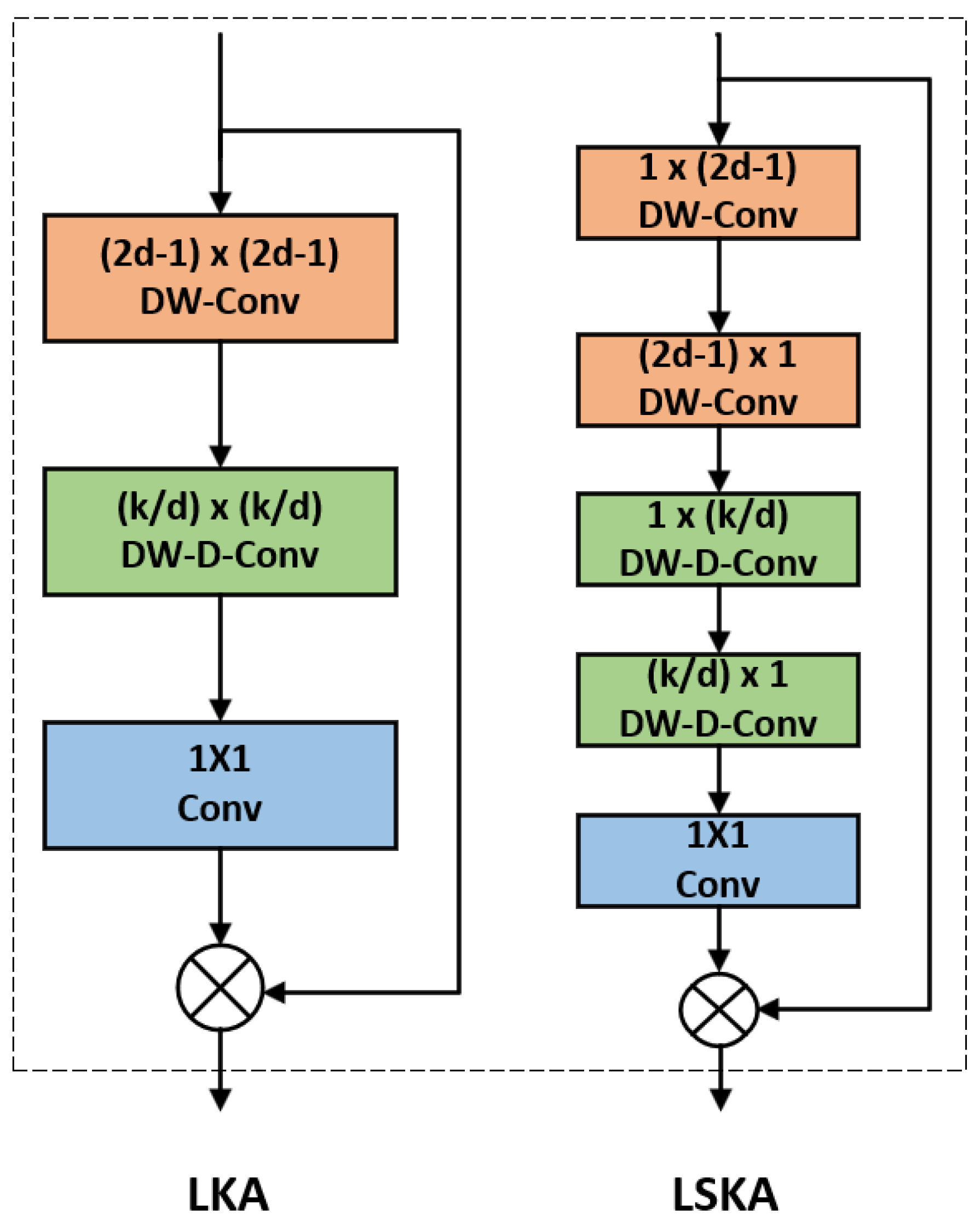
The LSKA attention mechanism is a lightweight and efficient spatial attention mechanism [
14]. Its core innovation lies in decomposing large-sized two-dimensional convolutional kernels into cascaded one-dimensional convolutions based on traditional large-kernel attention (LKA). This effectively resolves the quadratic explosive growth in computational and memory overhead caused by excessively large convolutional kernels, enabling the attention module of Visual Attention Networks (VAN) [
15] to utilize large convolutional kernels.
Figure 6 compares the network architectures of the LSKA and LKA attention mechanisms.In the figure,
k represents the maximum receptive field, and
d represents the expansion rate.
The LSKA module incorporates both horizontal and vertical convolutional layers, each responsible for extracting features along the horizontal and vertical directions of the input feature map. These layers generate preliminary attention maps, enabling the model to focus attention on critical regions within the image. Following the generation of these preliminary attention maps, spatial dilation convolutional layers with varying dilation rates are employed. This approach expands the receptive field without increasing computational cost, capturing richer contextual information and further refining the extraction of image features. Finally, a convolutional layer fuses the extracted features to generate the final attention map. This attention map undergoes element-wise multiplication with the original input feature map. Consequently, each element in the original feature map is weighted according to the attention map's values, amplifying significant features while suppressing less relevant ones.
Compared to traditional large convolutional kernel attention (using k×k convolutions as an example), the LSKA attention mechanism decomposes the two-dimensional convolutional kernel into cascaded horizontal (1×k) and vertical (k×1) one-dimensional convolutional kernels. This reduces computational complexity from O(k2) to O(k), decreases the number of parameters by 90%, significantly lowers memory requirements, and enhances the model's global context modeling capabilities and spatial perception abilities.
Assuming the input feature is,the computational process of the LSKA module can be expressed by the following equation:
Horizontal convolution(1×k):.
Vertical convolution(k×1):.
Spatial Attention Generation(1×1):;σ is the activation function.
Feature Adjustment:;denotes element-wise
multiplication (Hadamard product).
2.2.4. Wise-IoU v2 Loss Function
Wise-IoU v2 is a bounding box regression loss function based on a dynamic monotonic focusing mechanism [
16]. By introducing a Focal Loss-like focusing mechanism [
17] on top of Wise-IoU v1 and optimizing training stability through a dynamic normalization factor, it effectively reduces the impact of easy samples on the loss, enabling the model to focus more on difficult samples.
The Wise-IoU v2 formula is expressed as:
In the formula:is the focus parameter, reflecting the suppression strength for simple samples,;is the exponential moving average of ;Through the calculation of ;is the momentum parameter used for dynamically updating the normalized reference.Selecting as the normalization factor resolves the issue where the gradient gain r decreases as φIoU diminishes, leading to slow convergence during the latter stages of model training.Here, the gradient gain .
Wise-IoU v2, as an efficient bounding box regression loss function, employs a monotonic focusing mechanism and dynamic normalization factor to reduce the competitiveness of high-quality anchor boxes while minimizing harmful gradients from low-quality samples. This enables the model to focus more intently on optimizing difficult samples that are hard to regress, thereby enhancing overall detection accuracy. Additionally, it accelerates model convergence and improves robustness.
3. Experimental Setup
3.1. Dataset
The dataset used in this experiment was collected from municipal drainage pipe networks, comprising approximately 700 original images. To enhance the model's generalization capability, data augmentation techniques—including rotation, occlusion, and cropping—were applied to expand the dataset to 2,000 images [
18]. The dataset covers the following common pipeline defect types: fractures, holes, collapses, surface corrosion, deformation, spalling, cracks, joint displacements, and deterioration.Because of the extreme scarcity of individual defect types and to avoid the confusion of anchor box color during the detection stage, four kinds of defects, such as fracture, hole, collapse and bend, are labeled with the same label. Therefore, the final dataset contains seven label categories.To ensure objectivity and reliability in model evaluation, the dataset was divided into a training set and a validation set in an 8:2 ratio. The training set contains 1,600 images, and the validation set contains 400 images. This partitioning strategy supports robust model generalization.
Figure 7 illustrates representative examples of each defect category in the dataset.
3.2. Laboratory Facility Configuration
The experimental program used in this paper is based on the PyTorch 2.0.1 deep learning framework, corresponding to CUDA version 11.7, with Python 3.9.21 as the programming language. Furthermore, to ensure the rigor and completeness of the experimental results, the entire experiment was conducted using the same hardware device: a high-performance server equipped with an NVIDIA GeForce RTX 4090 GPU, 24GB of graphics memory, and running the Ubuntu 18.04 operating system.
3.3. Experimental Parameter Specifications
During the model training phase, to ensure training efficiency and the validity of training results, appropriate experimental parameters must be configured. The settings for some parameters in this experiment are as follows: The training epochs were set to 400. Image resolution was uniformly set to 640×640 pixels. The batch size was set to 64. The optimizer type was selected as SGD with momentum set to 0.937. Weight decay was set to 0.0005. The learning rate was set to 0.01. Data loading workers set to 8, random seed set to 0 to ensure experiment reproducibility, confidence threshold set to 0.5, and Intersection over Union (IoU) threshold set to 0.7.
After model training is completed, to evaluate the quality of training results and assess its performance, the experiment employs Mean Average Precision (mAP), Parameter quantities and computational cost (GFLOPs) as performance metrics. The calculation formulas are as follows:
In these formula, P represents Precision, R represents Recall, TP denotes the number of correctly detected instances, FP represents the number of false positives, FN indicates the number of missed detections, AP is the average precision, whose value is obtained by integrating the area under the P-R curve. mAP stands for mean average precision, a performance metric calculated as the arithmetic mean of AP values across all classes when the intersection-over-union ratio (IoU) between predicted and ground-truth boxes exceeds a specified threshold. n denotes the total number of target classes.
4. Results Analysis
4.1. Experimental Results
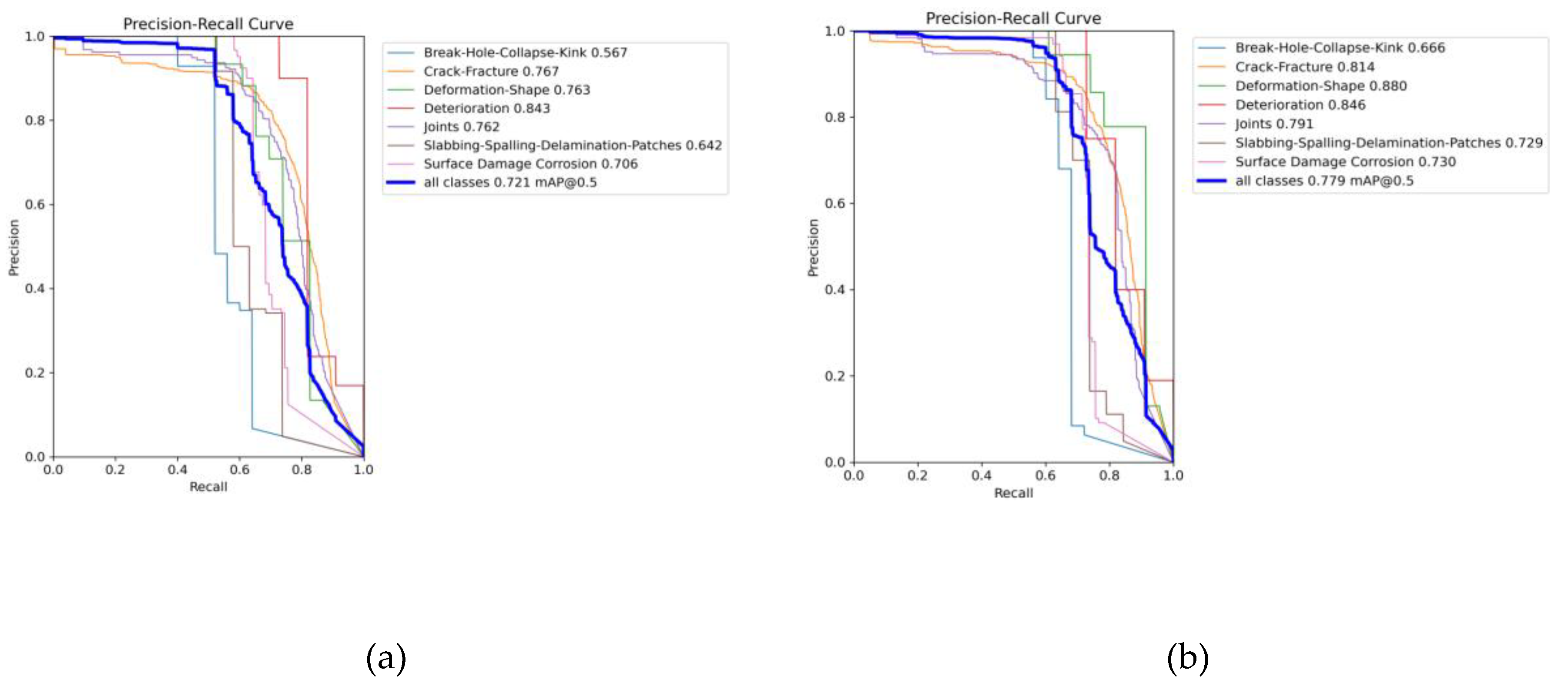
The experimental results indicate that the proposed FALW-YOLOv8 lightweight model demonstrates superior performance across all metrics compared to the YOLOv8 baseline. Specifically, the mean Average Precision (mAP50) increased by 5.8 percentage points, from 72.1% to 77.9%. The number of parameters was reduced by approximately 34.7%, from 3M to 1.96M, and the computational complexity (GFLOPs) decreased by about 30.9%, from 8.1G to 5.6G.
Figure 8 presents a comparison of the Precision-Recall (P-R) curves for defect detection before and after the improvement.
Comparing the P-R curves before and after the improvements reveals that the enhanced model achieves higher detection accuracy across all defect categories. Overall, the detection performance is more balanced, demonstrating an improved equilibrium between precision and recall.
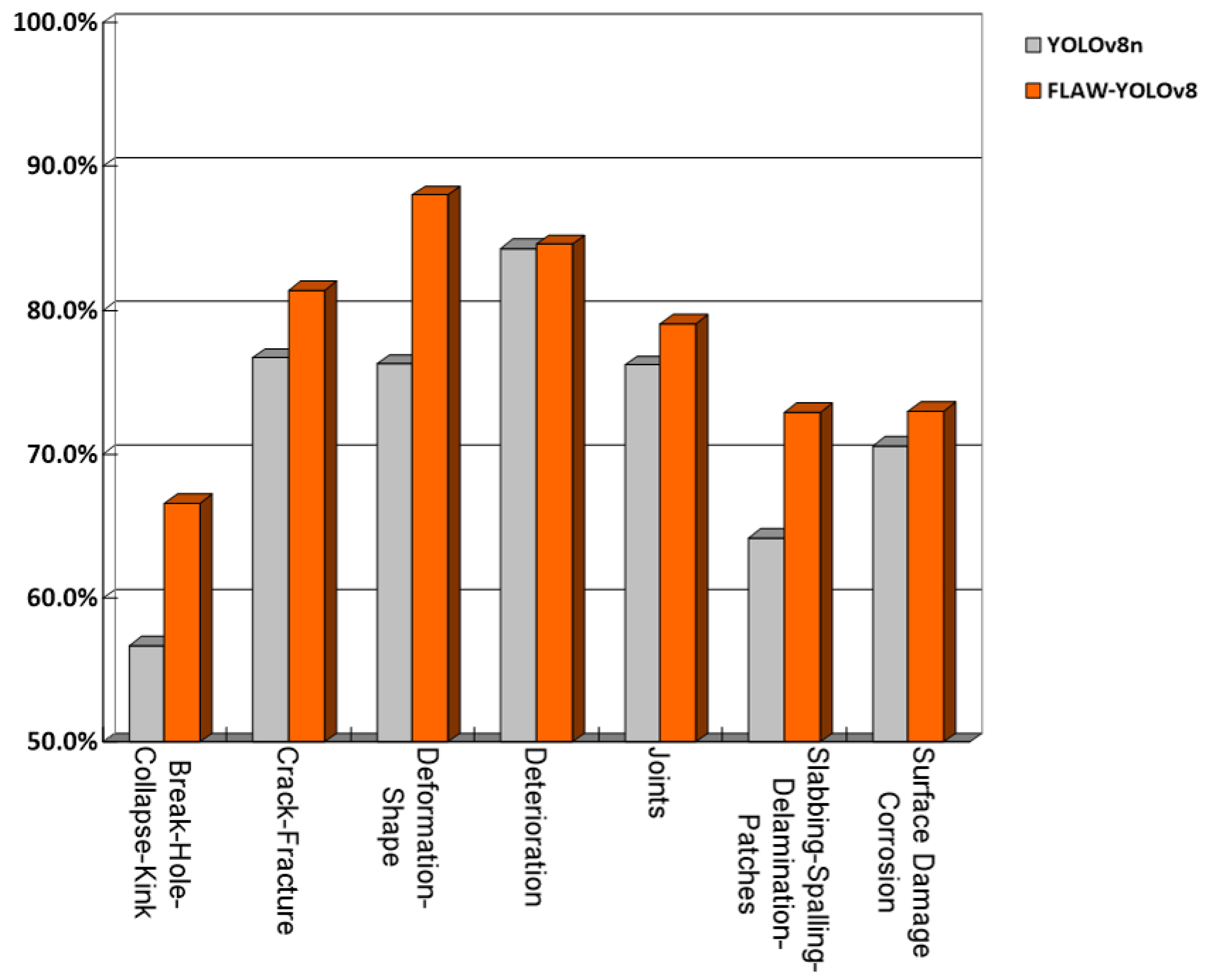
To more clearly illustrate the performance changes in defect detection across various categories before and after model improvements, a comparative histogram is provided as shown in
Figure 9.
4.2. Ablation Experiment
To verify that each individual improvement module positively contributes to the overall model, this experiment designed five ablation studies.Each study employed identical training parameters and environmental conditions, varying only the number of active improvement modules. The results are presented in
Table 1.
Analysis of the ablation experiment data reveals that the baseline YOLOv8 model achieves a mAP50 of 72.1%, with 3.00M parameters and 8.1G GFLOPs. After introducing the C2f-FasterBlock module, mAP50 improved to 73.4%, parameters decreased to 2.31M, and GFLOPs dropped to 6.4G. This demonstrates that the module effectively reduces computational complexity and parameter count while minimizing memory usage and enhancing the model's ability to extract key features. Further integration of the ADown module elevated mAP50 to 75.1%, reduced parameters to 1.89M, and lowered GFLOPs to 5.5G. This demonstrates that the module, through optimized combinations of asymmetric convolution kernels and adaptive channel mechanisms, effectively reduces model parameters and computational overhead while enhancing feature expression capabilities to capture richer semantic information. Subsequently, integrating the LSKA attention mechanism further elevated the model's mAP50 to 77.7%, though parameters and GFLOPs saw a slight increase. This demonstrates that the LSKA module significantly enhances the model's spatial perception of defects across different scales and its feature discrimination capabilities with minimal computational overhead, substantially improving detection accuracy. Finally, integrating the C2f-FasterBlock, ADown, LSKA, and Wise-IoU v2 modules slightly improved the model's mAP50 to 77.9%. This demonstrates that the Wise-IoU v2 loss function enhances the model's adaptability to complex scenes, improves localization accuracy, strengthens robustness, and elevates overall detection precision.
4.3. Model Comparison Experiment
To validate the effectiveness of the improved algorithm in pipeline defect detection tasks, this paper designed a model comparison experiment.Several mainstream object detection algorithms were selected for comparison,including the two-stage detection model Faster R-CNN,the one-stage detection models RetinaNet and SSD300,and common models from the YOLO series—YOLOv3-tiny, YOLOv5, YOLOv6, YOLOv8, YOLOv10n, and YOLOv11n. The experimental results are shown in
Table 2.
The results reveal that while the traditional two-stage detection model Faster R-CNN demonstrates good detection accuracy, its reliance on the Region Proposal Network (RPN) for object localization incurs high computational overhead and requires a large number of model parameters. Its relatively complex structure limits its application in lightweight scenarios. In contrast, one-stage detection models like RetinaNet and SSD300 enhance inference efficiency by directly predicting bounding boxes. However, they fail to achieve significant improvements in detection accuracy—SSD300 even showed a marked decline. Furthermore, both models exhibit weaker overall detection performance, particularly in complex scenes where they are susceptible to background interference. The widely adopted YOLO series models demonstrate exceptional advantages in lightweight design and real-time capabilities.Experimental results demonstrate that the proposed FALW-YOLOv8 model outperforms other reference models in pipeline defect detection tasks across performance, lightweight design, and computational efficiency. Regarding core detection accuracy, FALW-YOLOv8 achieves mAP50 and mAP50-95 scores of 77.9% and 48.9%, respectively. ranking first among all reference models for both metrics. Compared to the YOLOv8 baseline model, these represent improvements of 5.8 percentage points and 3.5 percentage points respectively. This demonstrates the model's enhanced stability in identifying targets across varying overlap levels (from low to high IoU), particularly excelling in complex scenarios involving small or occluded objects. In balancing target capture and classification reliability, this model achieves a recall rate of 67.1%, the highest among all reference models, representing a 3.3 percentage point improvement over the YOLOv8 baseline model. This effectively reduces the risk of missed detections. Simultaneously, the model maintains a high accuracy rate of 88.9%, effectively avoiding the sharp increase in false positive rates that often accompanies the pursuit of high recall. This achieves an optimal dual balance of low missed detections and low false positives. Regarding deployment adaptability, FALW-YOLOv8 features only 1.96 million parameters and a computational load (GFLOPs) as low as 5.6G. Both metrics rank lowest among all reference models, enabling efficient adaptation to resource-constrained scenarios such as embedded devices and mobile platforms. It also supports real-time inference on low-computational-power hardware.
4.4. Model Interpretability and Feature Visualization Analysis
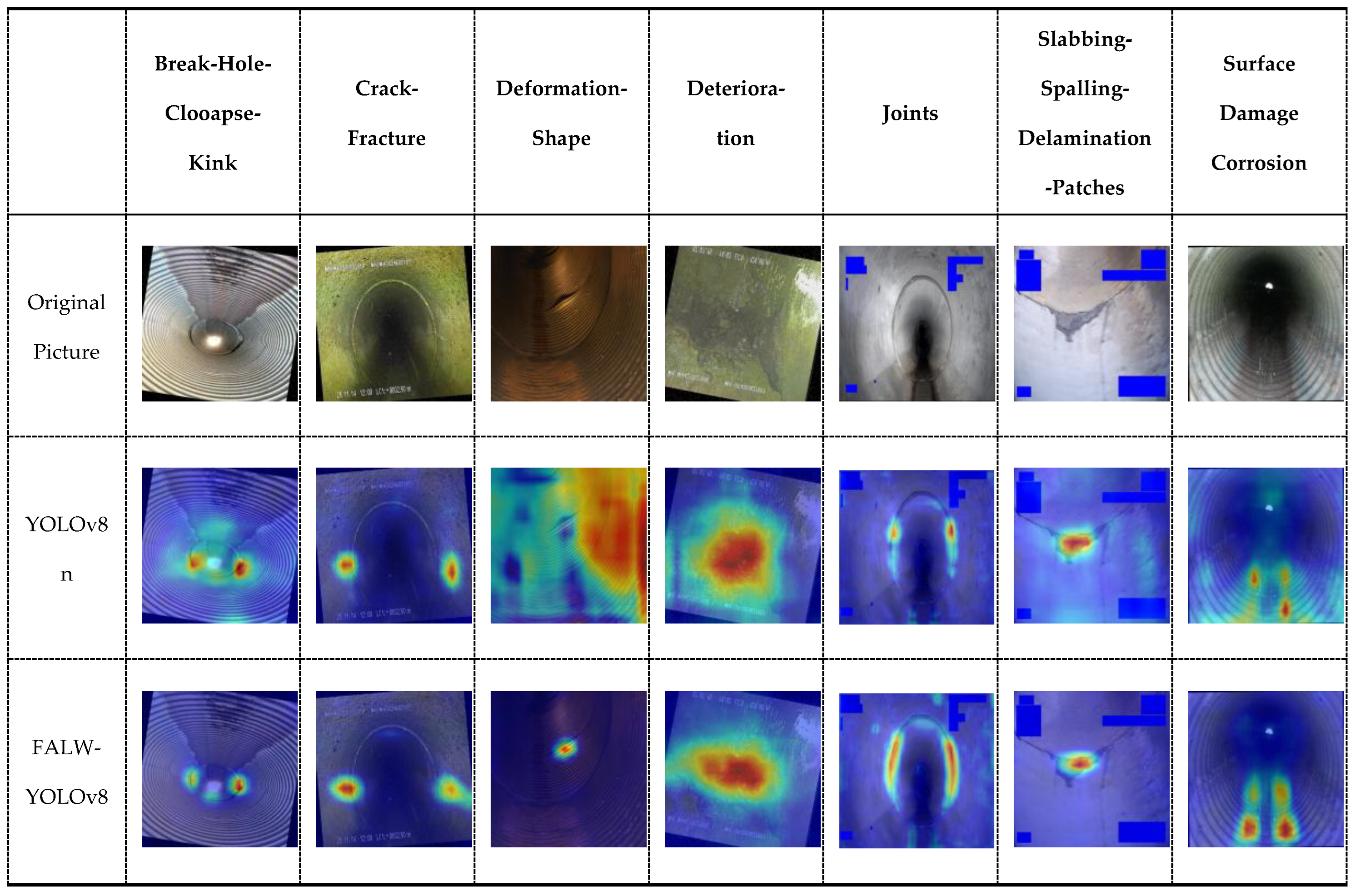
To further validate the feature extraction advantages of the improved model and validate its detection reliability in complex pipeline environments, this study utilized the EigenCAM algorithm to generate class-activation heatmaps, providing a qualitative analysis of the model's visual attention mechanism. The research systematically compared the feature activation patterns of the baseline YOLOv8 model and the FALW-YOLOv8 improved model across different defect categories. The experimental results are presented in
Table 3.
Observations indicate that the baseline model exhibits a certain degree of "feature divergence" and "background drift" when processing pipeline images characterized by regular textural backgrounds. Specifically, in categories such as "Deformation-Shape" and "Joints," the attention of the baseline model is frequently distracted by pipe wall corrugations or specular reflections, resulting in a failure to precisely focus on the defect subjects.
In contrast, the improved model demonstrates significantly superior spatial localization capabilities and interference resistance. Benefiting from the LSKA mechanism's capacity to capture long-range dependencies, the heatmaps generated by the improved model exhibit enhanced compactness and semantic alignment. The high-confidence regions (indicated in red) accurately cover irregular crack and deformation areas while effectively suppressing background noise. This visually demonstrates that the improved algorithm not only enhances detection accuracy but also successfully extracts highly discriminative key features within the defects, thereby evidencing robust performance and interpretability.
Author Contributions
Conceptualization, Qingchao Jiang and Lihua Sun; methodology, Huazhong Wang and Xuetao Wang; software, Qingchao Jiang; validation, Huazhong Wang,Lihua Sun and Xuetao Wang; formal analysis, Qingchao Jiang; investigation, Xuetao Wang; resources, Lihua Sun; data curation, Xuetao Wang; writing—original draft preparation, Xuetao Wang; writing—review and editing, Qingchao Jiang; visualization, Lihua Sun; supervision, Qingchao Jiang; project administration, Lihua Sun. All authors have read and agreed to the published version of the manuscript.