
Submitted:
09 December 2025
Posted:
10 December 2025
You are already at the latest version
Abstract
Assessing the stress–strain state around interacting mining excavations using the finite element method (FEM) is computationally expensive for parametric studies. This study evaluates tabular machine-learning surrogate models for the rapid prediction of full stress–strain fields in jointed rock. A dataset of 1000 parametric FEM simulations using the elastoplastic Hoek–Brown constitutive model was generated to train Random For-est, LightGBM, CatBoost, and Multilayer Perceptron (MLP) models based on geometric features. The results show that the best models achieve R2 scores of 0.96–0.97 for stress components and 0.99 for total displacements. LightGBM and CatBoost provide the op-timal balance between accuracy and computational cost, offering speed-ups of 15 to 70 times compared to FEM. While Random Forest yields slightly higher accuracy, it is re-source-intensive. Conversely, MLP is the fastest but less accurate. These findings demonstrate that data-driven surrogates can effectively replace repeated FEM simula-tions, enabling efficient parametric analysis and intelligent design optimization for mine workings.

Keywords:
surrogate modeling
; geomechanics
; machine learning
; AI-assisted design
; stress–strain fields
; mining excavations
; Hoek–Brown criterion
; gradient boosting
1. Introduction
The assessment of the stress–strain state (SSS) of fractured rock masses in the interaction zone of mining excavations is a central problem in geomechanics [1,2,3], directly affecting the safety and economic efficiency of engineering decisions [4,5]. The finite element method (FEM) remains the standard tool for solving this problem across a wide range of geotechnical applications [6,7,8]. However, in tasks requiring multiple recalculations—such as probabilistic analyses, parameter optimization, and the comparison of alternative design solutions within intelligent mining frameworks—direct use of FEM becomes computationally expensive. Every new configuration requires mesh regeneration and a full re-solution of the problem, and both meshing and computation remain the bottleneck even with automated workflows.
In this context, surrogate modeling based on machine learning (ML) has emerged as a promising alternative capable of rapidly approximating dependencies identified through FEM. Existing studies show successful applications of surrogate models primarily for predicting integral scalar indicators, such as tunnel stability coefficients in different geological conditions, bearing capacity of foundations, slope stability, and retaining structure performance [9,10,11,12,13]. In such works, the target variables typically represent single aggregated characteristics of system behavior.
In contrast, predicting full spatial fields of the SSS is a considerably more complex task, generally addressed using architectures designed for spatial data processing. One common approach represents geometry and output fields as images and applies convolutional neural networks (CNNs), including conditional generative adversarial networks (cGANs), which have demonstrated the ability to reproduce stress fields for complex geometries and boundary conditions [14,15,16]. Another approach represents the finite element mesh as a graph and uses graph neural networks (GNNs), such as MeshGraphNets, which can significantly accelerate FEM simulations in solid mechanics by operating directly on unstructured meshes [17,18,19]. Although highly accurate, these models require specialized data representations (images or graphs) and are often computationally demanding to implement in routine engineering practice.
To facilitate AI-assisted design in mining, the present study considers an alternative paradigm: encoding the physics of the problem directly into the feature space by designing a set of engineering (contextual) features that describe the mutual arrangement of nodes and excavations as well as the geometry of the system. This strategy enables the application of classical tabular ML algorithms—primarily tree-based ensembles—that are well suited for structured data and provide high computational performance [20]. However, the applicability and comparative efficiency of such algorithms specifically for reproducing full SSS fields around interacting mining excavations remain insufficiently investigated.
The aim of this study is to compare the effectiveness of surrogate models (Random Forest, LightGBM, CatBoost, MLP) for the rapid prediction of SSS fields around two interacting underground excavations based on FEM simulations.
The objectives of the study are as follows:
- To generate a parametric dataset of 1000 FEM simulations and develop an engineering feature space that reflects the geometry of the system and the spatial position of nodes relative to the excavations.
- To train and compare surrogate models in terms of accuracy (, MAE) and computational performance (training time, inference speed, model size, and learning curves).
- To evaluate model interpretability using permutation feature importance and to conduct qualitative validation of SSS fields (including plastic zones) against reference FEM results.
2. Materials and Methods
The research methodology (Figure 1) included: parametric FEM modeling to generate a synthetic dataset of simulations; extraction of SSS fields and construction of engineering features; splitting the dataset into training/validation/test subsets with cumulative subsamples for learning curves; hyperparameter optimization using Optuna and model training (Random Forest, LightGBM, CatBoost, MLP); followed by a comprehensive evaluation of model accuracy and computational efficiency.
2.1. Numerical Modeling
The dataset used for model training was generated by conducting a series of 1000 parametric simulations in a geotechnical finite element software package. To automate geometry generation, modification of input parameters, and extraction of simulation outputs, an application programming interface (API) controlled by a Python script was employed.
The computational model (Figure 2) represents a 50 × 50 m rock mass domain containing two parallel horseshoe-shaped underground excavations. The model dimensions were selected to eliminate the influence of boundary effects. The mechanical behaviour of the rock mass was simulated using an elastoplastic constitutive model with a Hoek–Brown yield criterion, developed for fractured rock masses [21,22]. Equivalent Mohr–Coulomb parameters were derived using the procedure proposed by Hoek and Brown [23].
The physical and mechanical properties adopted in the model are presented in Table 1. Input parameters for such constitutive models—including deformability characteristics and shear strength parameters—are typically derived from laboratory tests on rock specimens [24,25]. The computational domain was discretized using 15-node triangular finite elements with local mesh refinement around the excavation contours.
To identify nodes that reached the limiting shear state, a dimensionless relative shear stress parameter was used:
where is the magnitude of mobilized shear stresses along the local shear plane, and is the ultimate shear strength computed according to the Mohr–Coulomb criterion: .
Within this study, the parameters listed in Table 1 were kept constant, while six global parameters governing the geometry and relative position of the excavations were varied: horizontal spacing and vertical offset between excavation centres, as well as the width and height of each excavation. Parameter values were sampled from predefined uniform distributions. The variation ranges are presented in Table 2.
For each simulation, the following data were extracted from all nodes of the finite element mesh:
Basic features: nodal coordinates (X, Y).
Target variables: six components of the stress–strain state, including effective normal stresses (, ), shear stresses (), strain components (, , ), as well as total displacement ().
2.2. Feature Space and Its Construction
Since the original nodal coordinates (X, Y) do not provide ML models with explicit information about the geometry of the computational domain, and the global parameters alone are insufficient to capture dependencies explaining the target variables, a set of engineering (contextual) features was developed. These features supply the model with information about the spatial position of each node relative to the excavation contours and the overall system geometry. The full set of input features used for training is summarized in Table 3.
The average excavation width () and height () were computed as:
where, are the widths of the first and second excavation, and are their heights.
The aspect ratios (, ) and area ratio () were defined as:
The normalized distance () and shift () were defined as:
The normalized signed distance () was given by:
where is the feature value for node ; is the set of points forming the excavation contour; is the mean excavation width; and is a function returning +1 for rock mass nodes and –1 for excavation nodes.
The overlap index () was defined as:
where , are the minimum distances from node to the nearest points on the contours of the first and second excavation, respectively, and is the mean excavation width.
The curvature feature () was defined as:
where is the point on the excavation contour closest to node ; is the local curvature of the contour at point , estimated by approximating a local segment with a circular arc; and is a parameter controlling the decay rate of curvature influence.
The vertical projection feature () was defined as:
where is the vertical offset from node to the nearest point on the excavation contour; is the Euclidean distance to the same point; is a monotonically increasing function; and is a function that limits the final value to the range [–1, 1].
The density feature () was computed as:
where is the feature value for node ; is the set of nodes belonging to the excavated domain; and is the cardinality of this set.
Visualizations of the engineering feature fields for a test example are shown in Figure 3.
After constructing the feature set, each FEM simulation was treated as a separate sample. The collection of files was randomly shuffled once and split at the file level into training (70%), validation (15%) and test (15%) subsets. Based on the training subset, cumulative subsamples were formed as follows: for k ∈{1–10, 16, 24, 32, 40, 56, 72, 80, 160, 240, 320, 400, 480, 560, 640, 700}, datasets were created containing the first k training files. Each subsequent subsample included all samples from the previous one, which enabled consistent construction of learning curves.
2.3. Machine Learning Algorithms Considered
A separate surrogate model was trained for each of the seven target parameters. The study compared four regression algorithms widely applied in engineering prediction tasks:
Random Forest (RF). An ensemble method based on bagging [26]. The model consists of T independent decision trees, each trained on a bootstrap sample, while only a random subset of features is considered when splitting a node. The final prediction is obtained by averaging the outputs of all trees in the ensemble, as shown in Equation (14):
Gradient Boosting. An ensemble method that constructs a composition by sequentially adding weak learners trained to approximate pseudo-residuals [27]. At each iteration, a new model is fitted to a vector that is anti-parallel to the gradient of the loss with respect to the current ensemble prediction. For the mean squared error (MSE), pseudo-residuals coincide with standard residuals, and the ensemble is updated according to Equation (15):
where is the learning rate. Two high-performance implementations of gradient boosting were used in this work:
LightGBM [28], which accelerates tree construction via a histogram-based split-search algorithm;
CatBoost [29], which employs ordered boosting to mitigate prediction bias and provides built-in tools for handling categorical variables.
Multilayer Perceptron (MLP). A feed-forward fully connected neural network. Each layer performs an affine transformation of the input vector followed by a nonlinear activation (e.g., ReLU). The network parameters are optimized via backpropagation [30] and gradient-based optimization methods. The loss function includes an L2-regularization term , as defined in Equation (16):
For tree-based models (RF, LightGBM, CatBoost), input features were not normalized because decision-tree-based algorithms are inherently invariant to monotonic transformations of the feature space. For MLP, all features were normalized using StandardScaler. The normalization parameters were computed exclusively on the corresponding training subset and subsequently applied to both validation and test subsets, preventing information leakage from the test data into the training process.
2.4. Training Methodology and Evaluation Criteria
For each algorithm and each target variable, hyperparameter optimization was carried out using the Optuna framework [31], which implements Bayesian optimization methods. The optimization objective was the coefficient of determination () on the validation set. A uniform computational budget was imposed in this study: 2 hours of hyperparameter search for each algorithm–target pair.
In addition, the following assumption was adopted: hyperparameter optimization was performed once on the full training set, and the resulting optimal configuration was then used to train models on all smaller subsamples. This strategy was chosen to standardise the comparison conditions and reduce the total computational time. However, it should be noted that each subsample may in principle have its own locally optimal set of hyperparameters.
The experiments were conducted on a workstation running Windows 11 Pro with an AMD Ryzen 5–class CPU (6 cores, 12 threads), 32 GB DDR4 RAM, an NVIDIA GeForce RTX 4070 GPU (12 GB VRAM) and a 512-GB NVMe SSD. The GPU was used for training and inference of the MLP (PyTorch) and LightGBM models, while Random Forest and CatBoost were executed on the CPU. The MLP models were trained in a full-batch regime, so the maximum size of the training set for this architecture was limited to 400 simulation cases by the available hardware resources.
All computations were performed in 32-bit precision (single precision), as increasing the numerical precision did not improve the results but led to higher demands on computational resources.
The performance of the surrogate models was assessed and compared using five criteria:
- Global predictive accuracy: The primary metric was the coefficient of determination () computed on the held-out test set. The dependence of on the size of the training data was analysed to construct learning curves and to identify the saturation point of accuracy [26].
- Accuracy in critical zones: To evaluate the ability of the models to predict material behaviour near the limit state, an additional analysis was carried out. For a series of simulations with fixed excavation geometry but varying distance between the excavations, the model predictions were compared with reference values of , and at nodes that had entered the plastic state (. The evaluation metric was the mean absolute error (MAE).
-
Computational efficiency: Both training and inference (prediction) speed were assessed:
- training time required to fit the model on training sets of different sizes;
- inference time required to generate predictions of the stress–strain fields for a single simulation case from the test set. For the MLP and LightGBM models, these computations were performed on the GPU, whereas RF and CatBoost used the CPU.
- Model compactness: The physical size of the trained model file on disk (in megabytes) was measured as an indicator of storage and deployment requirements.
- Interpretability: The contribution of each input feature to the final prediction was quantified using the Permutation Feature Importance (PFI) method [26]. The method consists in measuring the drop in after random permutation of the values of a given feature on the test set.
3. Results
Figure 4 shows the dependence of on the training set size for each of the seven predicted stress–strain parameters, with separate curves for RF, LightGBM, CatBoost and MLP. The corresponding maximum values are summarised in Table 4.
The analysis demonstrates the high predictive capability of the developed surrogate models for the stress components (, , ) and the total displacement . For these quantities, the tree-based models exhibit a consistent increase in as the size of the training set grows, with the accuracy approaching saturation at approximately 300–400 FEM simulations. When trained on the full dataset, high final values are achieved, in particular 0.967 for (LightGBM, CatBoost) and 0.998 for (LightGBM, Random Forest, CatBoost).
A comparison of the algorithms shows that LightGBM, Random Forest and CatBoost provide similarly high performance for the stress components and . LightGBM yields the best results for and , Random Forest performs best for and , while for , and the differences between the three tree-based models are negligible. The MLP model is consistently less accurate than the tree-based algorithms in all cases.
The lowest values are obtained for the strain components, particularly for , where the maximum is 0.601.
Figure 5 presents the dependence of model training time on the number of training samples. The plots reveal fundamental differences in the scalability of the considered algorithms. The maximum training times are summarised in Table 5.
For the gradient-boosting models, the increase in computational cost is the most predictable and efficient. The training time of LightGBM on the full dataset is on the order of ≈130–170 s, while CatBoost requires ≈120–270 s depending on the target parameter.
Random Forest proves to be the most computationally demanding algorithm: for some target parameters, the maximum training time reaches ≈7.8–8.1 × 10³ s, i.e. roughly an order of magnitude higher than for the gradient-boosting models.
The MLP model trains faster than the other algorithms for small and medium training set sizes; however, after a certain threshold (around 160–240 files) the training time increases by an order of magnitude and reaches ≈1.2–2.6 × 10³ s at the maximum dataset size. This behaviour is likely related to the limitations of the available hardware resources and specifics of the training implementation.
In addition to accuracy and training time, an important practical aspect is the compactness of the trained models, i.e. the physical size they occupy on disk. Figure 6 shows the dependence of model size on the number of training samples, and the corresponding maximum values are reported in Table 6.
The MLP model is the most compact and is practically insensitive to the size of the training set: the file sizes remain in the range of ≈0.3–0.6 MB for all target parameters.
The gradient-boosting models differ substantially in compactness. The size of LightGBM models stabilises at ≈23–25 MB, whereas for CatBoost the model size after an initial growth reaches ≈70–160 MB, depending on the target parameter.
In contrast, the Random Forest models exhibit a pronounced and almost linear increase in size with the number of training samples, reaching several gigabytes on the full dataset.
A key indicator governing the applicability of surrogate models for rapid assessment tasks is the inference speed, i.e. the time required to generate predictions for new data. Figure 7 compares the prediction times of models trained on datasets of different sizes with the reference time of a single FEM simulation. The maximum inference times are summarised in Table 7.
The results indicate a substantial (one to two orders of magnitude) speed-up in prediction for most models compared with direct numerical simulation (4.86 s).
The highest and most stable prediction speed is achieved by the MLP: its inference time does not depend on the training set size and is ≈0.004–0.007 s, corresponding to a speed-up of about 700–1200 times relative to FEM.
The gradient-boosting models are also efficient. For LightGBM, the maximum inference time lies in the range ≈0.14–0.29 s, providing a speed-up of approximately 15–30 times. For CatBoost, the values are ≈0.07–0.15 s, which corresponds to a speed-up of about 30–70 times.
For Random Forest, a pronounced dependence of inference time on model size and complexity is observed. For some target parameters, the prediction time remains at 0.1–0.4 s (up to ≈40-fold speed-up), but for the shear components (, ) it increases to 8–16 s, making the inference comparable to or even slower than a direct FEM simulation and severely limiting the practical applicability of this algorithm.
To assess the ability of the models to correctly predict material behaviour near the limit state, an additional analysis was performed. The prediction accuracy was evaluated at nodes that had entered the plastic regime according to the volumetric Hoek–Brown (HB) criterion or had reached the limiting shear state on the excavation boundary (). The metric used was the mean absolute error (MAE), averaged over the three stress components.
Figure 8 shows the dependence of MAE on the distance between the excavations C. The training data covered the range m; therefore, the points at m and m characterise the behaviour of the models under extrapolation.
Within the training range ( m), the gradient-boosting models provide the best accuracy: the average MAE is 197.3 kPa for LightGBM and 217.1 kPa for CatBoost. Random Forest yields a slightly higher error level (245.52 kPa), and the worst result is obtained with MLP (358.2 kPa).
The behaviour of the models outside the training range shows the expected degradation in accuracy. When extrapolating to small distances ( m), where stress concentrations and non-linear effects are most pronounced, a sharp increase in error is observed for all models; a similar trend is seen for m.
To quantify the relative contribution of the input features to the model predictions, the Permutation Feature Importance (PFI) method was applied. The method consists in measuring the drop in after randomly permuting the values of a given feature on the test set; this drop is directly proportional to the importance of the feature. The results are shown in Figure 9, where the numerical values correspond to the normalised feature importance (in %).
The heatmaps reveal a high degree of consistency among the tree-based models (RF, LightGBM, CatBoost). For these algorithms, the main share of importance (on average about 70–75%) is attributed to the engineered features (, , , , etc.), whereas the raw coordinates X and Y account for the remaining ≈25–30%. For the normal components , , , , the contribution of the engineered features reaches 80–90%, while for the shear components and total displacement (, , ) their share is about 55–60%. At the same time, global parameters such as , , , , and show zero importance for all models.
In the updated setting, the MLP model preserves the general tendency of dominance of the engineered features, but redistributes importance differently. For most normal components (, , , ) and for the total displacement , the key predictor becomes , whose contribution reaches ≈45–55% of total importance, while the shares of and are noticeably lower than in the tree-based models (typically 3–15%). For the shear components (, ), the distribution is more balanced: X, and all retain a substantial influence.
To qualitatively assess the ability of the surrogate models to approximate the spatial distribution of the stress–strain fields, a visual comparison was performed for a randomly selected test case. As an illustration, Figure 10 shows triptychs for for each algorithm. Each triptych includes the reference field from the FEM simulation, the field predicted by the model, and the map of absolute errors . To improve readability and suppress the influence of rare outliers, the colour scale on the error maps is clipped at the 99th percentile of the error distribution.
The obtained absolute error maps are generally consistent with the values (Table 4). The largest discrepancies for all models are localised in the immediate vicinity of the excavation boundaries, whereas in the bulk of the rock mass the errors remain relatively small. For LightGBM and Random Forest, the errors are mainly concentrated near the contours, with Random Forest providing a slightly more accurate reproduction of the fields; CatBoost is characterised by artefacts in the form of radially diverging “rays” emanating from the excavations. In the case of MLP, a fundamentally different pattern is observed: for , the model fails to reproduce the detailed structure of the target field, and the predicted distributions are noticeably smoother than those of the tree-based models, which leads to an underestimation of local stress extrema around the excavations.
4. Discussion
The comparison shows that, in terms of the coefficient of determination , the best performance is achieved by the gradient-boosting models (LightGBM, CatBoost) and Random Forest [32]. At the same time, the qualitative analysis of the fields revealed differences in the error patterns: for gradient boosting (CatBoost in particular), numerical artefacts were observed (radial “rays”, non-physical elongated zones of concentration), whereas Random Forest more frequently reproduced field patterns closer to the reference FEM solutions. The MLP exhibited smoothing, accompanied by a loss of local extrema.
From the viewpoint of computational characteristics, fundamental trade-offs were identified. LightGBM and CatBoost train rapidly on the full dataset (≈130–170 s and ≈120–170 s, respectively), with model sizes of ≈18–25 MB (LightGBM) and ≈70–160 MB (CatBoost), and stable inference times of ≈0.14–0.29 s and ≈0.07–0.15 s. Random Forest proved to be the most resource-demanding: training time reaches ≈7.8–8.1 × 10³ s, model size grows to tens of gigabytes, and inference time for some target variables increases to 8–16 s, making these configurations comparable to or slower than a direct FEM run (4.86 s), which negates the advantage of using surrogates for real-time mining monitoring tasks The MLP provides the lowest inference latency (≈0.004–0.007 s, a speed-up of about 700–1200 times relative to FEM) with very compact models (≈0.5 MB), but it is less accurate than the tree-based models.
The permutation feature importance analysis showed that the tree ensembles rely primarily on engineering features , validating the proposed physics-informed approach. For the vertical components (, ), dominates (in total ≈50–65%); for , , and are particularly important; for , , the contribution of X is large; and for , Y and play a leading role. The high importance of geometric and positional features is typical for stability assessment problems and is consistent with previous studies [11,13,33].
The dependence of accuracy on the data volume exhibits saturation for most targets at ≈300–400 simulations (30–40% of the dataset); further increases in yield only limited improvements in R². For the strains, especially , the achieved values are lower, which indicates the need to enrich the feature space with descriptors more sensitive to local deformation effects. The analysis of accuracy in plastic zones (according to the Hoek–Brown criterion) confirmed that prediction errors increase significantly when the distance between excavations C goes beyond the training range ( m). This highlights the limited ability of the models to approximate behavior governed by the HB criterion outside the training domain—a critical consideration for safety assessments in mining design when solving extrapolation problems.
From a practical point of view, for rapid assessment and multi-scenario analysis, CatBoost and LightGBM are optimal in terms of the combination of accuracy, training time and model size, whereas MLP provides the lowest inference latency provided that adequate regularisation is applied. Although Random Forest can reproduce the stress–strain fields more faithfully than gradient boosting, its use is not justified for large datasets.
The practical advantages of the surrogate models are expected to be most significant for three-dimensional layouts, where a single FEM simulation may require hours or days. In such cases, surrogates can replace FEM in tasks involving a large number of forward evaluations, while FEM is retained for detailed verification. Typical examples include probabilistic analyses of pillar stability, optimization of mining excavation layouts, and routine screening of design alternatives within Digital Twin frameworks. For these applications, increasing the dimensionality of the problem primarily affects the cost of generating the training dataset, whereas the prediction time of the LightGBM, CatBoost, and MLP models remains essentially constant.
5. Conclusions
This study has demonstrated and systematically evaluated the applicability of classical tabular machine-learning algorithms for constructing surrogate models capable of predicting, with high accuracy and speed, the full stress–strain fields in a rock mass around a system of two interacting mining excavations.
It has been confirmed that tree ensembles (Random Forest, LightGBM, CatBoost) provide high predictive accuracy, reaching for the stress components and for the total displacements. The most important factor for model accuracy is the use of engineering features, whose importance is consistent with the physical pattern of stress distribution in jointed rock masses.
The comparative analysis revealed fundamental trade-offs between the algorithms suitable for intelligent design:
- The MLP offers the lowest inference latency (≈0.004–0.007 s, a speed-up of 700 to 1200 times relative to FEM) with compact models, but produces smoother fields with partial loss of local features.
- LightGBM and CatBoost provide the most balanced combination of accuracy and computational cost ( close to Random Forest, speed-up of 15 to 70 times relative to FEM), making them ideal for iterative design optimization.
- Random Forest yields fields closest to reference FEM solutions but is too resource-demanding for large-scale deployment.
It has been established that model accuracy saturates at ≈300–400 parametric simulations, allowing for the optimization of computational costs during data preparation. The analysis of the mean absolute error (MAE) in plastic zones showed that within the training range ( m), LightGBM attains the lowest error values. Outside this range, the error increases systematically, reflecting the limitations of data-driven models in extrapolation.
Overall, the proposed approach represents an effective tool for rapid stress–strain assessment at the design stage, substantially reducing computational costs. These properties make the proposed surrogates suitable as core components of probabilistic and optimization-based design workflows for underground mining. Large ensembles of scenarios can be evaluated using surrogate models, while detailed FEM analyses are reserved for critical cases. This division of roles allows engineers to account for parameter uncertainty and explore alternative layouts systematically, supporting the transition towards AI-assisted intelligent mining.
Author Contributions
Conceptualization, A.P.; methodology, A.P.; software, A.I.; validation, A.I.; formal analysis, A.I.; investigation, A.I.; resources, A.P.; data curation, A.I.; writing—original draft preparation, A.I.; writing—review and editing, A.P.; visualization, A.I.; supervision, A.P.; project administration, A.P. All authors have read and agreed to the published version of the manuscript.
Funding
This research received no external funding.
Data Availability Statement
The source code and datasets generated during the study will be made publicly available in a dedicated repository upon the article’s acceptance. During the peer-review process, the code and data can be provided to the Editor or reviewers upon request.
Acknowledgments
The authors would like to thank Empress Catherine II Saint Petersburg Mining University and the Department of Construction of Mining Enterprises and Underground Structures for providing the research infrastructure and academic environment that supported this work.
Conflicts of Interest
The authors declare no conflicts of interest.
Abbreviations
The following abbreviations are used in this manuscript:
| FEM: | Finite Element Method |
| ML: | Machine Learning |
| SSS: | Stress–Strain State |
| RF: | Random Forest |
| MLP: | Multilayer Perceptron |
| MAE: | Mean Absolute Error |
| HB: | Hoek–Brown |
References
- Demenkov, P.A.; Basalaeva, P. Regularities of Brittle Fracture Zone Formation in the Zone of Dyke Around Horizontal Mine Workings. Eng 2025, 6, 91. [Google Scholar] [CrossRef]
- Rysin, A.I.; Lebedeva, A.M.; Otkupshchikova, I.A.; Nurtdinov, A.S. Strength variation patterns in salt rocks owing to increased halopelite content. gzh 2025, 19–27. [Google Scholar] [CrossRef]
- Verbilo, P.E.; Karasev, M.A.; Shishkina, V.S. Geomechanical state of jointed rock pillar with the account of softening behaviour. gzh 2025, 41–47. [Google Scholar] [CrossRef]
- Basalaeva, P.V.; Kuranov, A.D. Influence of dip angle of lithologically nonuniform interburden on horizontal mine opening stability during driving. MIAB 2024, 3, 17–30. [Google Scholar] [CrossRef]
- Trushko, V.L.; Baeva, E.K. Substantiation of rational parameters of mine support system for underground roadways in difficult geological conditions. MIAB 2023, 55–69. [Google Scholar] [CrossRef]
- Belgueliel, F.; Fredj, M.; Saadoun, A.; Boukarm, R. Finite Element Analysis of Slope Failure in Ouenza Open-Pit Iron Mine, NE Algeria: Causes and Lessons for Stability Control. Journal of Mining Institute 2024, 268, 576–587. [Google Scholar]
- Demenkov, P.A.; Romanova, E.L. Regularities of Plastic Deformation Zone Formation Around Unsupported Shafts in Tectonically Disturbed Massive Rock. Geosciences 2025, 15, 23. [Google Scholar] [CrossRef]
- Trushko, V.L.; Baeva, E.K.; Blinov, A.A. Experimental Investigation on the Mechanical Properties of the Frozen Rocks at the Yamal Peninsula, Russian Arctic. Eng 2025, 6, 76. [Google Scholar] [CrossRef]
- Jearsiripongkul, T.; Keawsawasvong, S.; Thongchom, C.; Ngamkhanong, C. Prediction of the Stability of Various Tunnel Shapes Based on Hoek–Brown Failure Criterion Using Artificial Neural Network (ANN). Sustainability 2022, 14, 4533. [Google Scholar] [CrossRef]
- Kashyap, R.; Chauhan, V.B.; Kumar, A.; Jaiswal, S. Machine Learning-Based Stability Assessment of Unlined Circular Tunnels under Surcharge Loading. Asian J Civ Eng 2023, 25, 2553–2566. [Google Scholar] [CrossRef]
- Keawsawasvong, S.; Seehavong, S.; Ngamkhanong, C. Application of Artificial Neural Networks for Predicting the Stability of Rectangular Tunnels in Hoek–Brown Rock Masses. Front. Built Environ. 2022, 8, 837745. [Google Scholar] [CrossRef]
- Lai, V.Q.; Kounlavong, K.; Keawsawasvong, Suraparb; Wipulanusat, W.; Jamsawang, P. Physics-Based and Data-Driven Modeling for Basal Stability Evaluation of Braced Excavations in Natural Clays. Heliyon 2023, 9, e20902. [Google Scholar] [CrossRef]
- Nguyen, D.K.; Nguyen, P.T.; Ngamkhanong, C.; Keawsawasvong, S.; Lai, V.Q. Bearing Capacity of Ring Footings in Anisotropic Clays: FELA and ANN. Neural Computing and Applications 2023, 35, 10975–10996. [Google Scholar] [CrossRef]
- Jiang, H.; Nie, Z.; Yeo, R.; Farimani, A.B.; Kara, L.B. StressGAN: A Generative Deep Learning Model for Two-Dimensional Stress Distribution Prediction. Journal of Applied Mechanics 2021, 88, 051005. [Google Scholar] [CrossRef]
- Nie, Z.; Jiang, H.; Kara, L.B. Stress Field Prediction in Cantilevered Structures Using Convolutional Neural Networks. Journal of Computing and Information Science in Engineering 2020, 20, 011002. [Google Scholar] [CrossRef]
- Yang, Z.; Yu, C.-H.; Buehler, M.J. Deep Learning Model to Predict Complex Stress and Strain Fields in Hierarchical Composites. Science Advances 2021, 7. [Google Scholar] [CrossRef]
- Pfaff, T.; Fortunato, M.; Sanchez-Gonzalez, A.; Battaglia, P.W. Learning Mesh-Based Simulation with Graph Networks. 2020. [Google Scholar]
- Wu, J.; Du, C.; Dillenburger, B.; Kraus, M.A. Fast Prediction of Stress Distribution: A GNN-Based Surrogate Model for Unstructured Mesh FEA; Block, P., Boller, G., De Wolf, C., Pauli, J., Kaufmann, W., Eds.; International Association for Shell and Spatial Structures (IASS), 2024. [Google Scholar]
- Zhai, H. Stress Predictions in Polycrystal Plasticity Using Graph Neural Networks with Subgraph Training. Comput Mech 2025, 76, 387–408. [Google Scholar] [CrossRef]
- Wang, H.; Qiu, W.; Wang, H.; Li, J.; Li, X.; Zhou, B.; Xue, S.; Xiuxing, Z. A Machine Learning Method for Finite Element Stress Recovery Based on Feature Variables of Coordinate and Displacement. Mech. Solids 2025, 60, 720–736. [Google Scholar] [CrossRef]
- Hoek, E.; Brown, E.T. Empirical Strength Criterion for Rock Masses. J. Geotech. Engrg. Div. 1980, 106, 1013–1035. [Google Scholar] [CrossRef]
- Hoek, E.; Brown, E.T. The Hoek–Brown Failure Criterion and GSI – 2018 Edition. Journal of Rock Mechanics and Geotechnical Engineering 2019, 11, 445–463. [Google Scholar] [CrossRef]
- Hoek, E.; Brown, E.T. Practical Estimates of Rock Mass Strength. International Journal of Rock Mechanics and Mining Sciences 1997, 34, 1165–1186. [Google Scholar] [CrossRef]
- Gospodarikov, A.P.; Trofimov, A.V.; Kirkin, A.P. Evaluation of Deformation Characteristics of Brittle Rocks beyond the Limit of Strength in the Mode of Uniaxial Servohydraulic Loading. Journal of Mining Institute 2022, 256, 539–548. [Google Scholar] [CrossRef]
- Korshunov, V.A.; Pavlovich, A.A.; Bazhukov, A.A. Evaluation of the Shear Strength of Rocks by Cracks Based on the Results of Testing Samples with Spherical Indentors. Journal of Mining Institute 2023, 262, 606–618. [Google Scholar] [CrossRef]
- Breiman, L. Random Forests. Machine Learning 2001, 45, 5–32. [Google Scholar] [CrossRef]
- Friedman, J.H. Greedy Function Approximation: A Gradient Boosting Machine. Ann. Statist. 2001, 29, 1189–1232. [Google Scholar] [CrossRef]
- Ke, G.; Meng, Q.; Finley, T.; Wang, T.; Chen, W.; Ma, W.; Ye, Q.; Liu, T.-Y. LightGBM: A Highly Efficient Gradient Boosting Decision Tree. Proceedings of the Advances in Neural Information Processing Systems 30 (NIPS 2017) 2017, Vol. 30, 3149–3157. [Google Scholar]
- Prokhorenkova, L.; Gusev, G.; Vorobev, A.; Dorogush, A.V.; Gulin, A. CatBoost: Unbiased Boosting with Categorical Features. Advances in neural information processing systems 2018, 31. [Google Scholar] [CrossRef]
- Rumelhart, D.E.; Hinton, G.E.; Williams, R.J. Learning Representations by Back-Propagating Errors. Nature 1986, 323, 533–536. [Google Scholar] [CrossRef]
- Akiba, T.; Sano, S.; Yanase, T.; Ohta, T.; Koyama, M. Optuna: A Next-Generation Hyperparameter Optimization Framework. In Proceedings of the Proceedings of the 25th ACM SIGKDD International Conference on Knowledge Discovery & Data Mining, Anchorage AK USA, July 25 2019; ACM, 2019; pp. 2623–2631. [Google Scholar]
- Grinsztajn, L.; Oyallon, E.; Varoquaux, G. Why Do Tree-Based Models Still Outperform Deep Learning on Tabular Data? Advances in neural information processing systems 2022, 35, 507–520. [Google Scholar] [CrossRef]
- Jitchaijaroen, W.; Wipulanusat, W.; Keawsawasvong, S.; Chavda, J.T.; Ramjan, S.; Sunkpho, J. Stability Evaluation of Elliptical Tunnels in Natural Clays by Integrating FELA and ANN. Results in Engineering 2023, 19, 101280. [Google Scholar] [CrossRef]
Figure 1.
Flowchart of the research methodology.
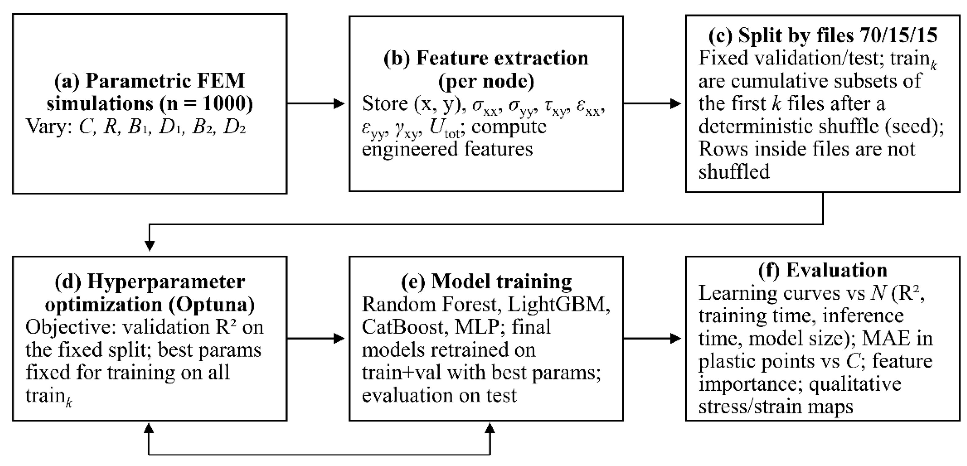
Figure 2.
Computational model.
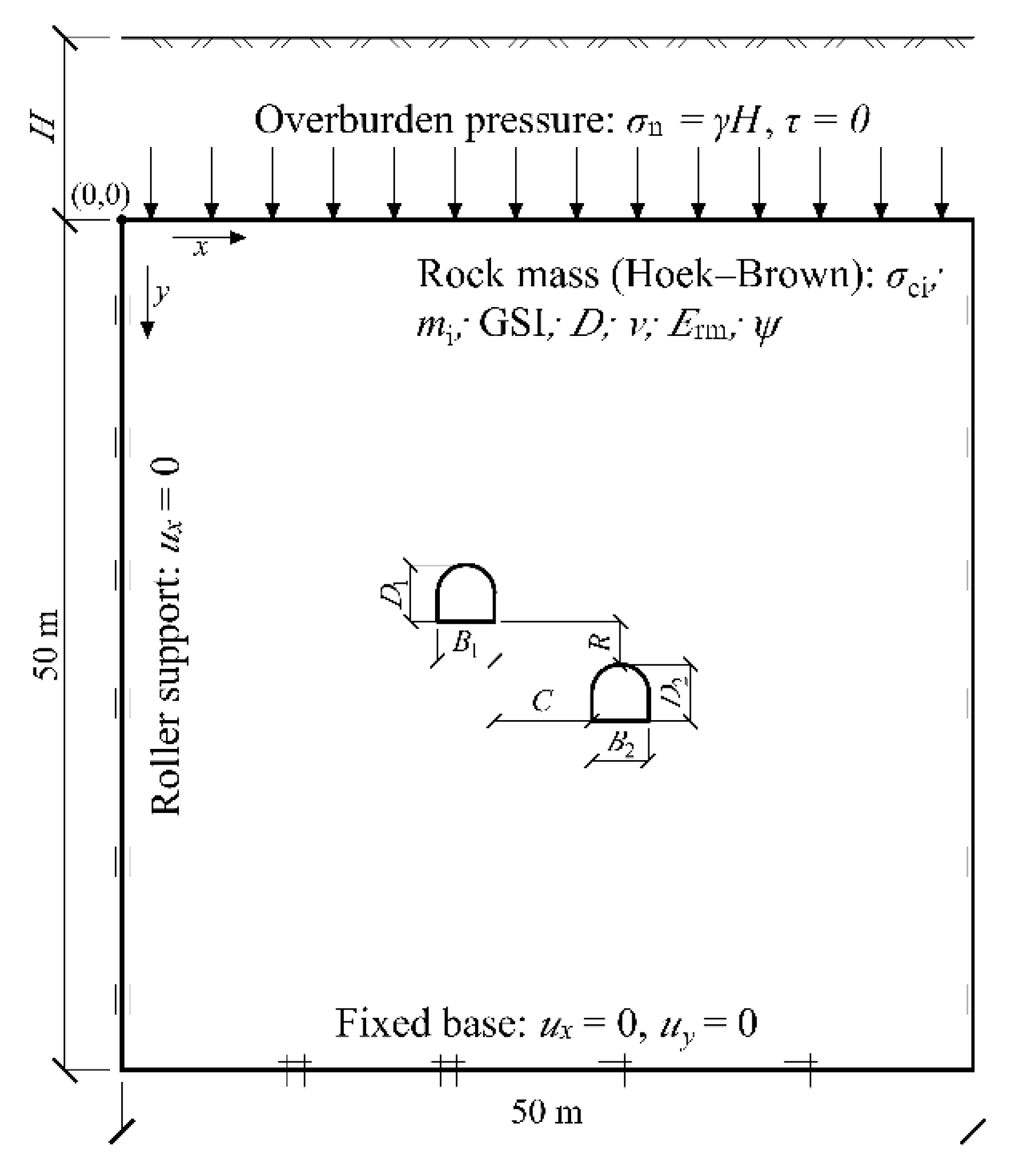
Figure 3.
Visualization of engineering feature fields for a test example: (a) Curvature; (b) Density_Excavated_Distances; (c) Overlap_Index; (d) Signed_Dist_Norm; (e) Vertical_Projection.
Figure 3.
Visualization of engineering feature fields for a test example: (a) Curvature; (b) Density_Excavated_Distances; (c) Overlap_Index; (d) Signed_Dist_Norm; (e) Vertical_Projection.
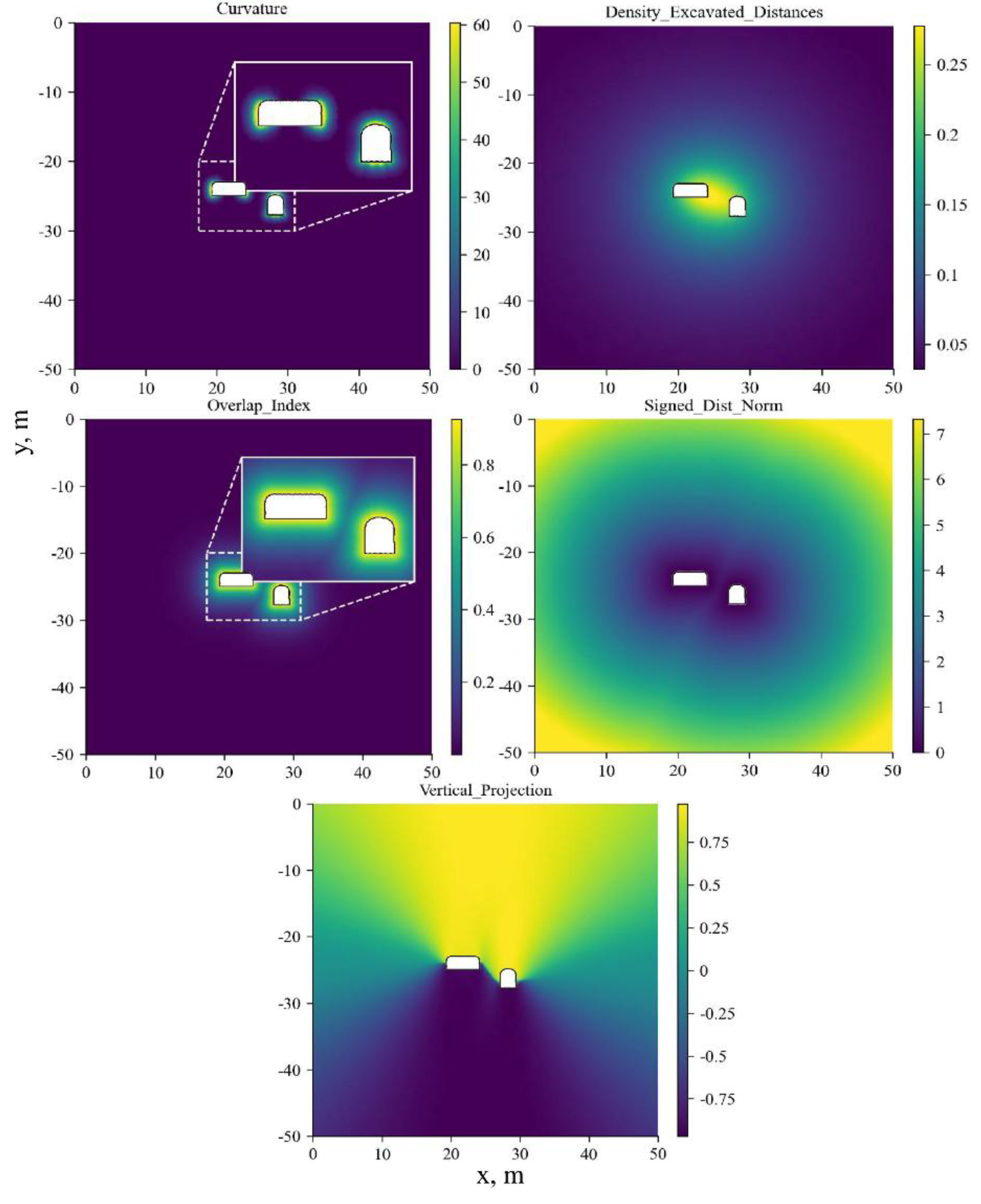
Figure 4.
Dependence of R² on the training set size for predicting: (a) ; (b) ; (c) ; (d) ; (e) ; (f) ; (g) (X-axis in logarithmic scale).
Figure 4.
Dependence of R² on the training set size for predicting: (a) ; (b) ; (c) ; (d) ; (e) ; (f) ; (g) (X-axis in logarithmic scale).
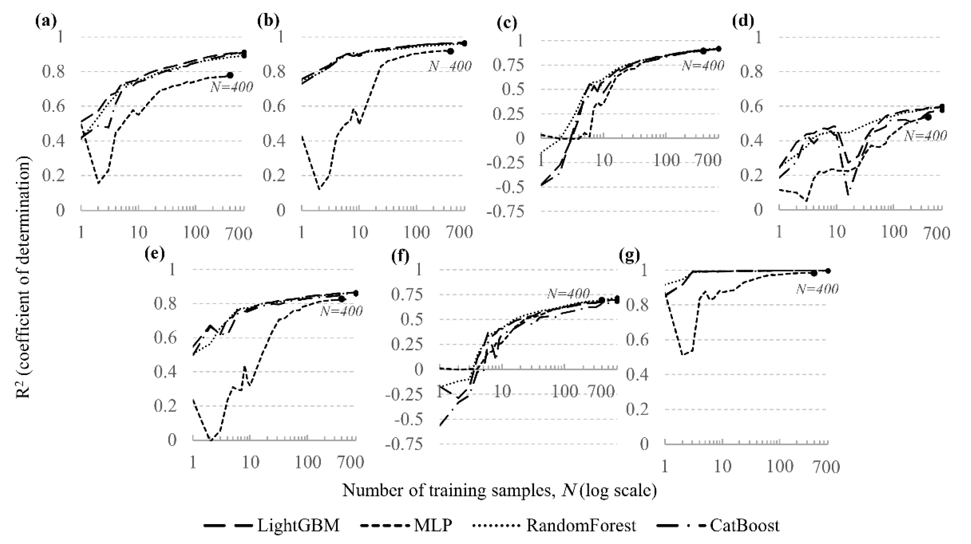
Figure 5.
Dependence of model training time on the number of training samples (FEM simulations) for the target parameters: (a) ; (b) ; (c) ; (d) ; (e) ; (f) ; (g) (X- and Y-axes in logarithmic scale).
Figure 5.
Dependence of model training time on the number of training samples (FEM simulations) for the target parameters: (a) ; (b) ; (c) ; (d) ; (e) ; (f) ; (g) (X- and Y-axes in logarithmic scale).
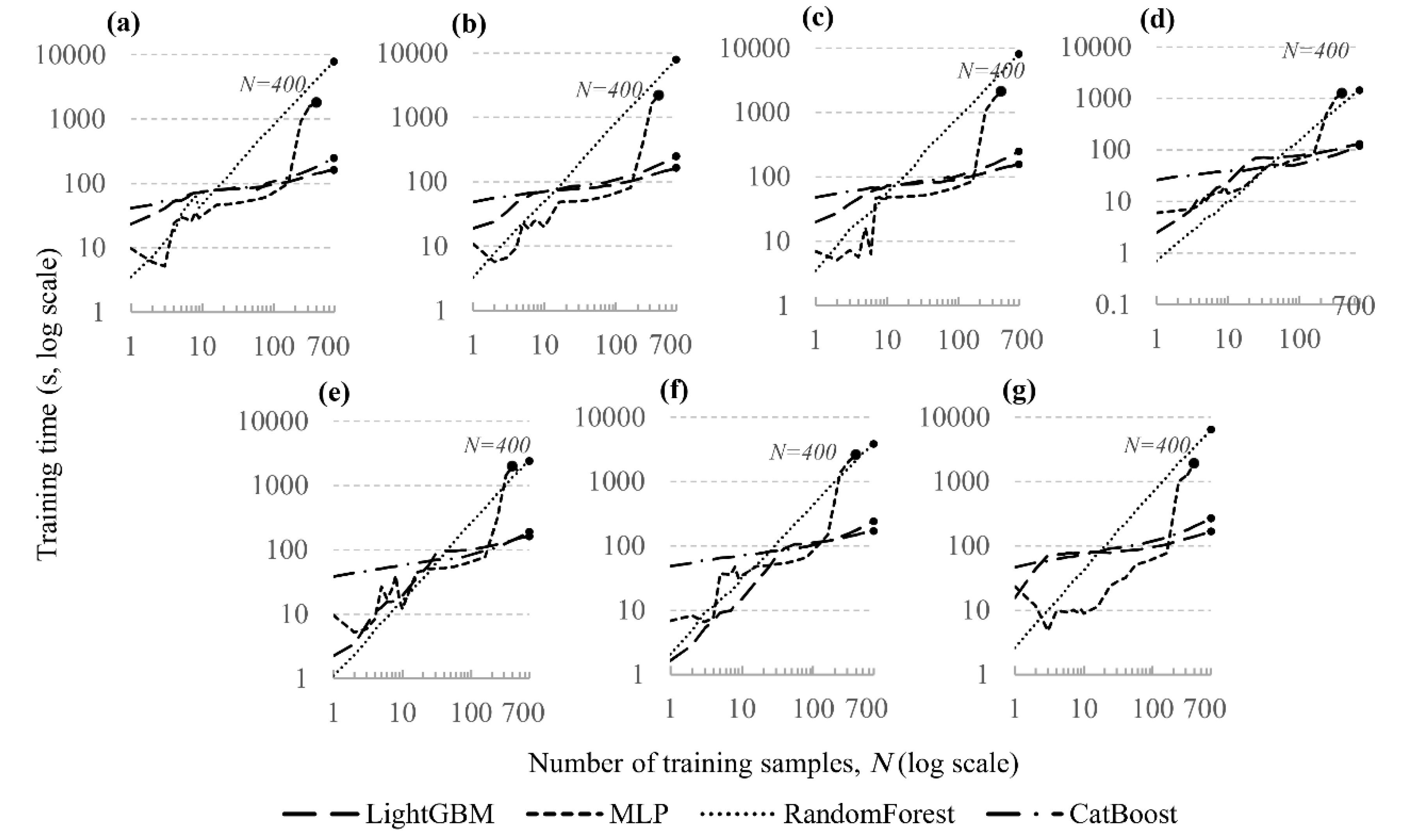
Figure 6.
Dependence of trained model file size (in megabytes) on the number of training samples (FEM simulations) for the target parameters: (a) ; (b) ; (c) ; (d) ; (e) ; (f) ; (g) (X- and Y-axes in logarithmic scale).
Figure 6.
Dependence of trained model file size (in megabytes) on the number of training samples (FEM simulations) for the target parameters: (a) ; (b) ; (c) ; (d) ; (e) ; (f) ; (g) (X- and Y-axes in logarithmic scale).
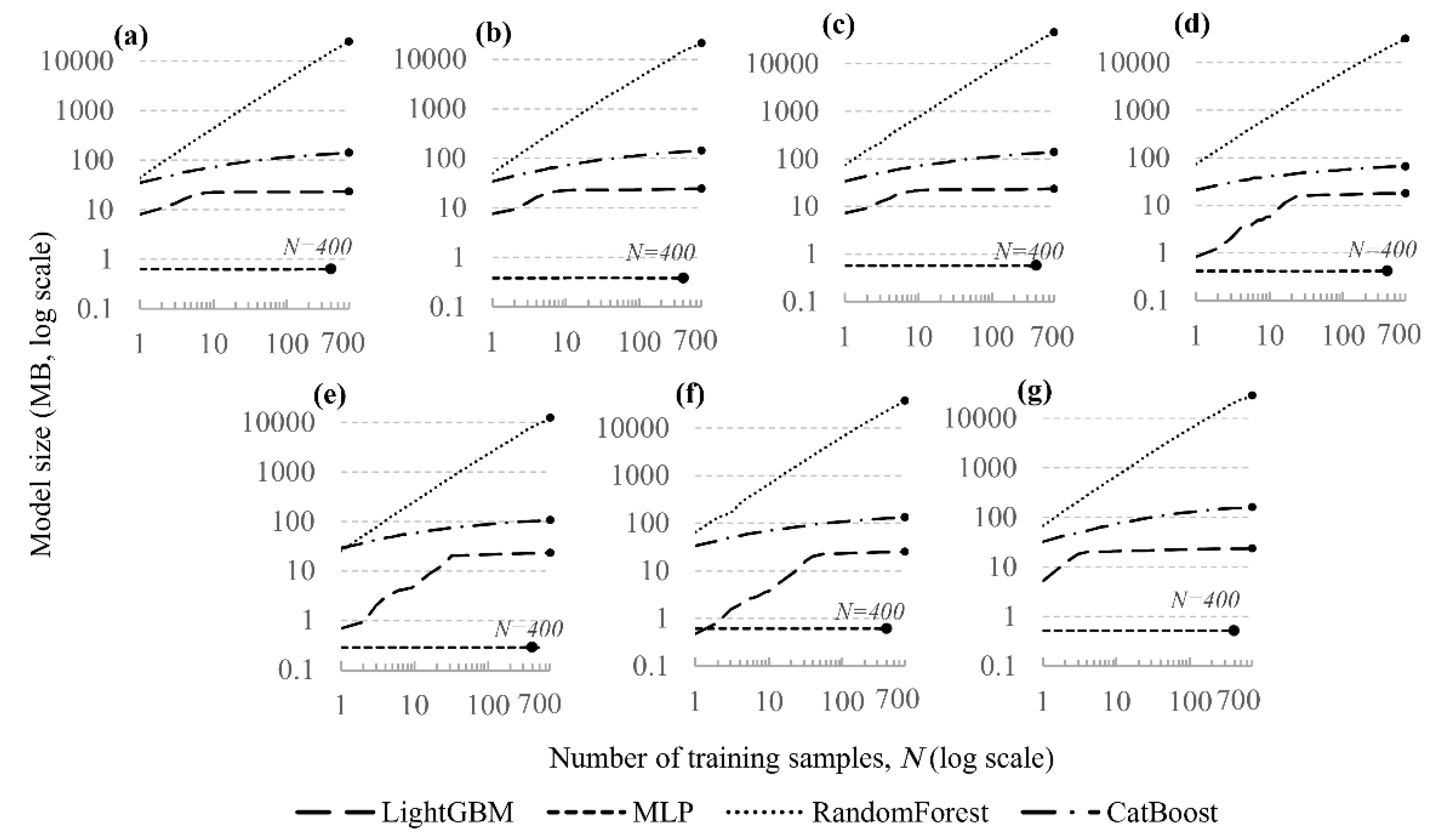
Figure 7.
Dependence of inference (prediction) time on the number of training samples (FEM simulations) for the target parameters: (a) ; (b) ; (c) ; (d) ; (e) ; (f) ; (g) (Y-axis in logarithmic scale).
Figure 7.
Dependence of inference (prediction) time on the number of training samples (FEM simulations) for the target parameters: (a) ; (b) ; (c) ; (d) ; (e) ; (f) ; (g) (Y-axis in logarithmic scale).
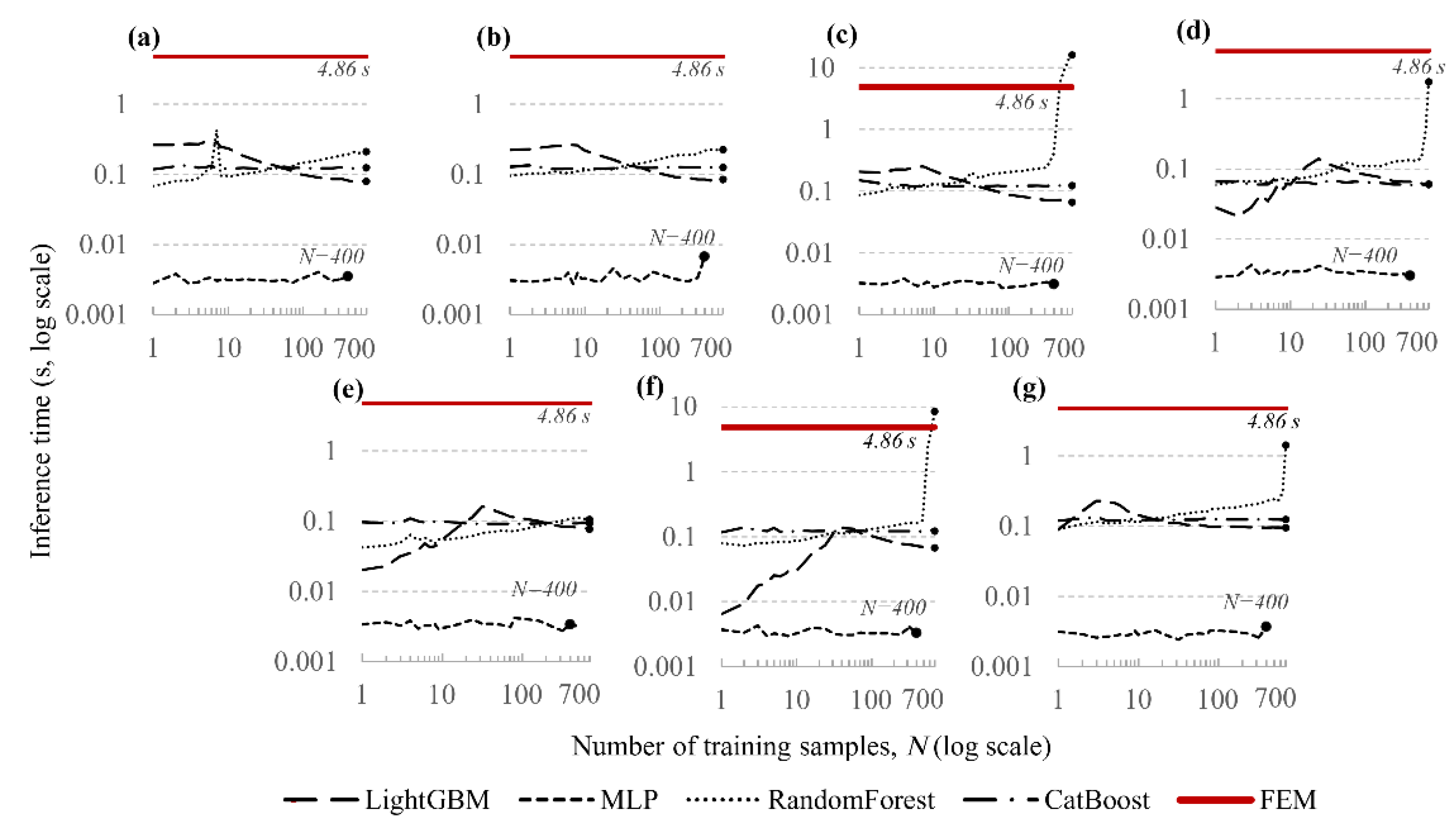
Figure 8.
Dependence of mean absolute error (MAE) of stress prediction in plastic points on the distance between excavations: (a) ; (b) ; (c)
Figure 8.
Dependence of mean absolute error (MAE) of stress prediction in plastic points on the distance between excavations: (a) ; (b) ; (c)
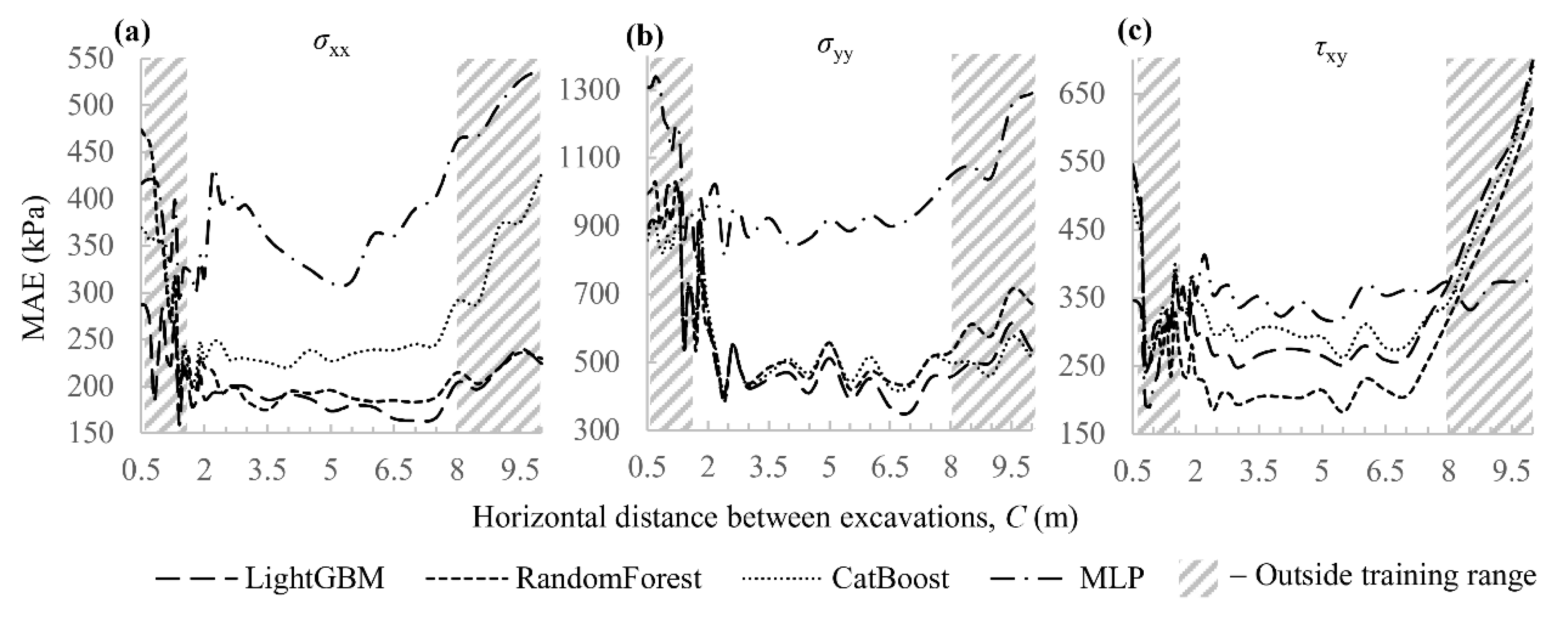
Figure 9.
Heatmaps of relative feature importance (Permutation Feature Importance) for the models: (a) CatBoost; (b) LightGBM; (c) MLP; (d) Random Forest.
Figure 9.
Heatmaps of relative feature importance (Permutation Feature Importance) for the models: (a) CatBoost; (b) LightGBM; (c) MLP; (d) Random Forest.
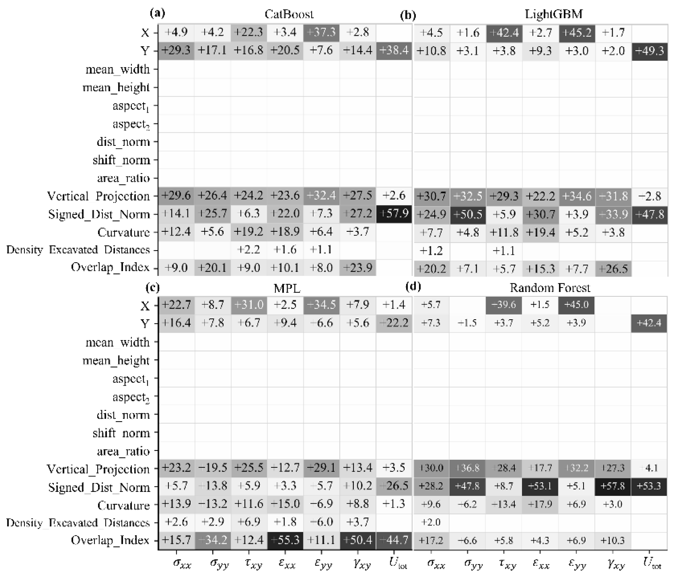
Figure 10.
Qualitative analysis of prediction results for the test case when predicting (kPa) for the models: (a) CatBoost; (b) LightGBM; (c) MLP; (d) Random Forest.
Figure 10.
Qualitative analysis of prediction results for the test case when predicting (kPa) for the models: (a) CatBoost; (b) LightGBM; (c) MLP; (d) Random Forest.
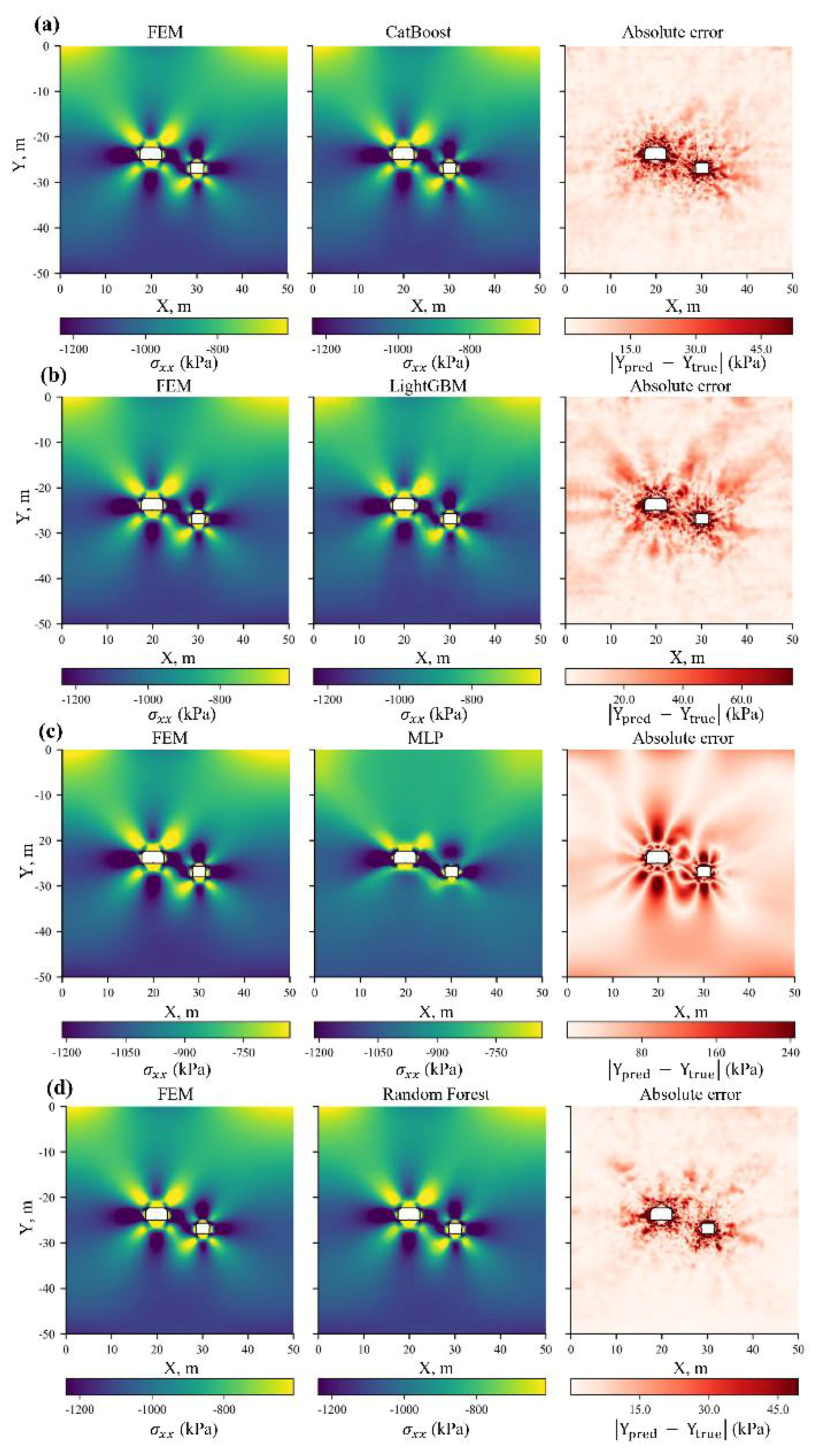

Table 1.
Rock mass parameters used in the model.
| Parameter | Symbol | Value | Unit |
| Unit weight | γsat | 25.4 | kN/m³ |
| γunsat | 23.0 | kN/m³ | |
| Geological Strength Index | GSI | 50 | — |
| Depth of excavation | H | 118 | m |
| Hoek–Brown constant for intact rock | mi | 15 | — |
| Disturbance factor | D | 0.5 | — |
| Dilatancy angle | ψmax | 4.0º | deg |
| Uniaxial compressive strength of intact rock | |σci| | 83356 | kN/m2 |
| Equivalent Young’s modulus of rock mass | Erm | 4408261 | kPa |
| Poisson’s ratio | ν | 0.2 | — |
| Model width | — | 50 | m |
| Model height | — | 50 | m |
Table 2.
Variable geometric parameters of the FEM model.
| Parameter | Symbol | Range | Unit |
| Horizontal distance between excavations | C | 1.0–8.0 | m |
| Vertical offset between excavations | R | -4.0–4.0 | m |
| Width of excavation 1 | B1 | 2.0–5.0 | m |
| Height of excavation 1 | D1 | 2.0–3.0 | m |
| Width of excavation 2 | B2 | 2.0–5.0 | m |
| Height of excavation 2 | D2 | 2.0–3.0 | m |
Table 3.
Input features for the machine learning models.
| Formula | Feature | Feature group |
| – | X, Y | Nodal coordinates |
| 2, 3 | mean_width, mean_height | Derived global parameters |
| 4,5 | aspect1, aspect2 | |
| 6 | area_ratio | |
| 7 | dist_norm | |
| 8 | shift_norm | |
| 9 | Signed_Dist_Norm | Engineering (contextual) features |
| 10 | Overlap_Index | |
| 11 | Curvature | |
| 12 | Vertical_Projection | |
| 13 | Density_Excavated_Distances |
Table 4.
Maximum coefficient of determination () values for each model and target parameter.
| Model | Stresses | Strains | Utot | ||||
| σxx | σyy | σxy | εxx | εyy | γxy | ||
| LightGBM | 0.912 | 0.967 | 0.914 | 0.601 | 0.865 | 0.702 | 0.998 |
| MLP | 0.778 | 0.920 | 0.893 | 0.536 | 0.826 | 0.690 | 0.984 |
| RandomForest | 0.892 | 0.960 | 0.919 | 0.594 | 0.865 | 0.716 | 0.998 |
| CatBoost | 0.910 | 0.967 | 0.914 | 0.579 | 0.859 | 0.685 | 0.998 |
Table 5.
Maximum training times (s) for each model and target parameter.
| Model | Stresses | Strains | Utot | ||||
| σxx | σyy | σxy | εxx | εyy | γxy | ||
| LightGBM | 164 | 166 | 157 | 131 | 162 | 171 | 168 |
| MLP | 1787 | 2189 | 2097 | 1252 | 1985 | 2604 | 1893 |
| RandomForest | 7790 | 7961 | 8111 | 1445 | 2402 | 3872 | 6477 |
| CatBoost | 249 | 251 | 249 | 121 | 191 | 243 | 271 |
Table 6.
Maximum file sizes of trained models (MB) for each model and target parameter.
| Model | Stresses | Strains | Utot | ||||
| σxx | σyy | σxy | εxx | εyy | γxy | ||
| LightGBM | 23.3 | 24.3 | 23.5 | 18.0 | 23.3 | 25.3 | 23.7 |
| MLP | 0.6 | 0.4 | 0.6 | 0.4 | 0.3 | 0.6 | 0.5 |
| RandomForest | 24716.1 | 21406.5 | 45946.1 | 31379.1 | 12435.2 | 37147.7 | 29298.6 |
| CatBoost | 140.9 | 143.9 | 139.9 | 67.4 | 107.3 | 134.0 | 161.7 |
Table 7.
Maximum inference times (s) for each model and target parameter.
| Model | Stresses | Strains | Utot | ||||
| σxx | σyy | σxy | εxx | εyy | γxy | ||
| LightGBM | 0.292 | 0.264 | 0.251 | 0.140 | 0.163 | 0.138 | 0.229 |
| MLP | 0.004 | 0.007 | 0.004 | 0.004 | 0.004 | 0.004 | 0.004 |
| RandomForest | 0.429 | 0.225 | 15.967 | 1.744 | 0.111 | 8.474 | 1.425 |
| CatBoost | 0.134 | 0.135 | 0.150 | 0.071 | 0.109 | 0.139 | 0.136 |
Disclaimer/Publisher’s Note: The statements, opinions and data contained in all publications are solely those of the individual author(s) and contributor(s) and not of MDPI and/or the editor(s). MDPI and/or the editor(s) disclaim responsibility for any injury to people or property resulting from any ideas, methods, instructions or products referred to in the content. |
© 2025 by the authors. Licensee MDPI, Basel, Switzerland. This article is an open access article distributed under the terms and conditions of the Creative Commons Attribution (CC BY) license (http://creativecommons.org/licenses/by/4.0/).
Copyright: This open access article is published under a Creative Commons CC BY 4.0 license, which permit the free download, distribution, and reuse, provided that the author and preprint are cited in any reuse.


