
Submitted:
08 December 2025
Posted:
09 December 2025
You are already at the latest version
Abstract
Multiple wide–area radio surveys report a source–count dipole whose amplitude exceeds the purely kinematic expectation inferred from the CMB dipole by a factor of ∼ 3–4, while remaining aligned with the CMB dipole direction. This tension, now detected at ≳ 5σ when combining NVSS, RACS–low and LoTSS–DR2, challenges the vanilla ΛCDM picture in which the radio dipole is dominated by Doppler and aberration effects with only a small clustering contribution. In this paper we present a quantitative implementation of Future–Mass Projection (FMP) gravity as a potential explanation of this anomaly. FMP is a diffeomorphism–invariant, bilocal, time–nonlocal extension of GR in which the effective source is a causal projection of the baryonic energy–momentum tensor along a finite, advanced horizon on a closed time path. On cosmological scales the theory can be parametrised by a scale– and time–dependent modification of the Poisson equation, μ(a, k), and lensing response, G(a, k), that are determined by the Fourier transform of the covariant kernel. We make three key advances compared to previous work. First, we provide an explicit mapping from an “entropic” Newtonian kernel, defined as the Hessian of a coarse–grained entropy functional in the space of disc and large–scale density configurations, to the cosmological response functions μ(a, k) and G(a, k). This leads naturally to a two–lobe scale dependence, with μ(a, k) < 1 on quasi–linear scales k ∼ 0.02–0.2 hMpc−1 and μ(a, k) > 1 on ultra–large scales k ≲ 0.01 hMpc−1, thereby reconciling a modest 10–15% suppression of fσ8 with an ultra–large–scale growth boost. Second, we fix the kernel parameters (ΔT, η, k1, k0) using two independent data sets: low–redshift redshift–space distortion measurements of fσ8 and galaxy rotation curves. This yields a single family of CTP kernels that already satisfies Solar–System, PPN and GW– speed constraints, and mildly alleviates the S8 tension. Third, using these pre–determined kernels, we compute the ultra–large–scale clustering boost factor BULS that enters the radio source–count dipole. We model the selection function W(z) and linear bias b(z) for NVSS, RACS–low and LoTSS–DR2, and evaluate the relevant integrals for BULS(ΔT, η, k0), propagating uncertainties from the kernel parameters and the source populations. For the kernel that best fits fσ8 and rotation curves we obtain a blind prediction RFMP ≡ dobs/ dkin = 3.2 ± 0.4, to be compared with the combined radio–dipole measurement Robs = 3.67 ± 0.49. A simple χ2 comparison shows that the anomaly is naturally reproduced within FMP without invoking particle dark matter, while remaining consistent with current large–scale structure and background probes. We discuss degeneracies, parameter–space constraints and the status of competing explanations for the radio–dipole excess.
Keywords:
dark matter
; modified gravity
; nonlocal gravity
; future–mass projection
; radio dipole
; large–scale structure
; cosmological principle
1. Introduction
Evidence from galaxy rotation curves, gravitational lensing and the cosmic microwave background (CMB) indicates that of the matter in the Universe is nonluminous and nonbaryonic.[1,2] The standard CDM model accounts for these observations with a cold, collisionless dark matter (DM) component and a cosmological constant, all gravitating according to General Relativity (GR). While the model fits many data sets remarkably well, the particle nature of DM remains unknown despite intensive searches.[3,4,5] At the same time, small–scale tensions and an emerging suppression of late–time structure growth (the so–called tension) motivate a closer look at the gravitational framework itself.
Modified gravity and nonlocal extensions of GR have been explored as alternatives or complements to particle DM.[6,7,8,9,10,11] Future–Mass Projection (FMP) gravity belongs to the latter class: it replaces particle DM with a causal, advanced projection of the baryonic energy–momentum tensor along a finite horizon on a closed time path (CTP).[12] At the covariant level, the Einstein tensor remains unchanged, but the effective source receives a nonlocal contribution from future segments of baryonic worldlines, subject to strict guardrails that preserve diffeomorphism invariance, conservation and local tests of gravity.
In this work we apply a quantitatively specified implementation of FMP to the cosmic radio–source dipole. In an isotropic universe, the differential number counts of extragalactic radio sources acquire a kinematic dipole due to our motion with respect to the cosmic rest frame. Its amplitude is given by [16,17]
where is our velocity relative to the CMB rest frame, x is the slope of the source counts and the spectral index. In CDM the observed dipole is expected to be well described by plus a small clustering term from large–scale structure.[18,19]
Analyses of NVSS, TGSS, WISE quasars and more recently RACS–low and LoTSS–DR2 instead find a radio–source dipole whose amplitude exceeds by a factor of –4 while remaining aligned with the CMB dipole direction.[20,21,22,23] A recent combined analysis using an improved estimator and joint modelling of multi–component sources finds[23]
which we take as our reference value.
The aim of this paper is not to claim that FMP must be the correct explanation, but to show that within a single, covariant, nonlocal framework one can:
- (i)
- consistently construct a kernel that preserves the CDM background, CMB physics, PPN parameters and GW speed;
- (ii)
- mildly suppress on quasi–linear scales while enhancing growth on ultra–large scales;
- (iii)
- predict, with kernel parameters fixed by other observables, a radio–dipole amplitude compatible with the observed excess.
We emphasise from the outset that our implementation of the scale dependence in is phenomenological: we model the response of the full covariant kernel by a small number of effective modes that capture its leading principal components in k–space. The underlying microscopic kernel is unique; the two–lobe representation is an economical effective description of its dominant projections.
The paper is organised as follows. Section ?? briefly reviews the DM landscape and situates FMP among nonlocal gravity models. Section 3 summarises the covariant FMP kernel, the CTP construction and the mapping to and the lensing response . Section 4 introduces the entropic organisation of the Newtonian kernel and its connection to the cosmological kernel. In Section 5 we fix the kernel parameters using and rotation–curve data. Section 6 reviews the radio–dipole measurements and presents our modelling of and . Section 7 contains the quantitative computation of and the resulting prediction for , including uncertainties. Section 8 discusses alternative explanations, systematics and future tests. We conclude in Section 9.
2. Theoretical Landscape and the Place of FMP
2.1. Particle Dark Matter and Late–Time Tensions
In the standard picture, cold dark matter is a pressureless fluid of weakly or feebly interacting particles with negligible thermal velocities at late times.[1] WIMP models obtain the observed relic abundance via thermal freeze–out, axions via the misalignment mechanism, and sterile neutrinos via nonthermal production.[3,4,5]
Despite the empirical success of CDM, several issues remain. Direct, indirect and collider searches have not produced an unambiguous detection. On small scales, cores in dwarf galaxies, the diversity of rotation curves and the missing–satellites problem invite either astrophysical or gravitational explanations. On quasi–linear scales, many weak lensing and redshift–space distortion data sets prefer a lower value of than inferred from Planck, suggesting a suppression of growth at relative to the vanilla model.[24]
These tensions may be resolved within particle DM, modified initial conditions or systematic uncertainties, but they also open a window for modified gravity and nonlocal effects.
2.2. Modified Gravity and Nonlocal Extensions
Modified Newtonian dynamics (MOND) postulates a breakdown of Newton’s law at accelerations below a characteristic scale , reproducing flat rotation curves and the baryonic Tully–Fisher relation with minimal parameters.[6] Relativistic completions like TeVeS address lensing and cosmology but face challenges for clusters and CMB.[7] Scalar–tensor–vector theories can fit some galaxy and cluster data without DM, though their full cosmological viability remains under investigation.[8] Emergent gravity attempts to derive gravity as an entropic response of microscopic degrees of freedom and predicts additional “dark” contributions tied to de Sitter entropy.[9]
Nonlocal gravity models add explicitly nonlocal terms to the gravitational action, often involving inverse d’Alembertians acting on curvature scalars.[10,11] These constructions can mimic DM or dark energy without new particles but must be carefully engineered to respect causality, conservation laws and Solar–System tests.
2.3. Future–Mass Projection (FMP)
FMP gravity introduces a different sort of nonlocality: the effective source is a causal, finite–horizon projection of the baryonic energy–momentum tensor along advanced segments of worldlines.[12] The Einstein equation retains its standard form,
but the effective source is given by
where is a bilocal kernel defined on a CTP segment that runs from t to along timelike geodesics, and is the baryonic energy–momentum tensor. The kernel obeys:
- (i)
- Finite horizon: vanishes for proper–time separations .
- (ii)
- Zero DC: For homogeneous configurations, the kernel integrates to zero, so the background expansion is not altered by inhomogeneous terms.
- (iii)
- Causality and conservation: The CTP construction and diffeomorphism invariance ensure , , and PPN parameters identical to GR in the appropriate limit.[12]
Cosmologically, one can define a “path–B” implementation in which the homogeneous matter density includes an FMP contribution in a fixed ratio to baryons, chosen such that the background expansion matches that of a reference CDM model.[14] All genuinely new physics is then encoded in the inhomogeneous kernel acting on structure, which can be parametrised in linear theory by scale– and time–dependent response functions and , as we describe next.
3. Covariant CTP Kernel and Cosmological Response
3.1. Linear Response and Two–Lobe
In the scalar sector of cosmological perturbations, the impact of FMP on structure growth can be captured by two functions: a modification of the Poisson equation, , and a modification of the lensing potential, :
where and are the Bardeen potentials and is the comoving matter density contrast. The function replaces the symbol commonly used in the literature to avoid confusion with the surface density introduced later.
For a finite–horizon CTP kernel, the linear response in Fourier space can be written as
where is the Fourier transform of the time– and space–dependent kernel, and is a dimensionless normalisation parameter inherited from the covariant kernel.
In the previous version of this work we adopted a single window function and wrote , which only allows a unidirectional deviation from unity. This is too restrictive to simultaneously suppress on quasi–linear scales and enhance growth on ultra–large scales. In the present version we instead write
where
- is a broad window peaked at with , representing a mild suppression of gravity on quasi–linear scales –;
- is a narrow window peaked at ultra–large scales with , responsible for the ULS boost.
Both windows obey a zero–DC condition in real space, reflecting the underlying guardrail of the covariant kernel.
A simple choice that captures these features is
with and . The time dependence is encoded in and , which vanish at recombination and grow only at late times to preserve CMB physics. In this parametrisation, a single underlying CTP kernel can generate a two–lobe : the quasi–linear suppression is associated with one effective mode of the kernel, and the ULS boost with another, both originating from the same covariant structure through its entropic organisation (Section 4.2). At the present level, however, we treat and their characteristic scales and time dependence as an effective description of the full kernel, not as a unique prediction.
The linear growth factor then obeys
with primes denoting derivatives with respect to . For small deviations, we can treat the impact perturbatively:
with the scale factor at recombination. By choosing and , one can obtain on (suppressing ) and on (enhancing ULS clustering), resolving the apparent contradiction between late–time growth suppression and radio–dipole enhancement.
Model complexity. The parametrisation in Eq. (8) introduces several effective degrees of freedom: from the covariant kernel, and from the two scale windows, and the time envelopes . In practice, the envelopes are chosen from a restricted functional family tied to the finite projection horizon and are fixed by the fit to and the requirement that at early times. The effective dimensionality of the problem is therefore higher than in CDM, where linear growth is controlled mainly by , but still modest compared to fully general modified–gravity parametrisations. We explicitly fix from , and from the requirement that the ULS lobe does not affect galaxy scales and remains compatible with lensing, before computing the radio–dipole prediction.
3.2. Lensing Response
The lensing response is obtained from the same covariant kernel by considering the combination that enters light deflection. In the simplest implementation we take
with constants controlling the relative lensing response of the two lobes. In the kernel family used below we choose such that galaxy–scale lensing and Bullet–Cluster–like lensing morphologies are matched without particle DM, while CMB lensing remains close to the CDM prediction.[15]
4. Entropic Organisation of the Newtonian Kernel
4.1. Entropy Functional and Hessian in Configuration Space
On sub–horizon, weak–field scales, the covariant kernel reduces to a Newtonian kernel acting on quasi–static mass distributions. For axisymmetric discs with surface density profiles and total baryonic mass
we define a coarse–grained functional that plays the role of an entropy–like potential. Motivated by information–theoretic considerations and the behaviour of fluctuations in self–gravitating systems, we consider
with
where is the fluctuation around a background profile , is a radial weight and an inverse covariance kernel. With the sign convention , maxima of physical entropy correspond to minima of S, so that the Hessian of S is positive semi–definite at equilibrium.
The entropic FMP kernel is defined as
where
and is a dimensionless normalisation fixed by matching to the covariant kernel. For exponential discs and Gaussian choices of w and , one can impose a radial zero–DC condition,
ensuring that the entropic response redistributes the effective mass but does not add a homogeneous monopole.[13]
4.2. From Entropic Kernel to
The bridge between the entropic Newtonian kernel and the cosmological response proceeds in three conceptual steps:
- (a)
- Embed the 2D disc kernel into a 3D kernel , e.g. by assuming axial symmetry and a vertical scale height , so that corresponds to a smoothed 3D density .
- (b)
- Take the 3D Fourier transform,and perform a principal–component analysis (PCA) of the kernel in k–space over a physically relevant range of environments.
- (c)
- Identify the leading principal components with effective windows and in Eq. (8), with their time dependence inherited from the underlying CTP horizon and the late–time envelope of the advanced kernel.
In practice, the PCA step is numerical and environment–dependent; a full implementation is beyond the scope of this paper and will be presented elsewhere. Here we treat and as phenomenological stand–ins for the dominant eigenmodes of in k–space, chosen such that they reproduce the desired quasi–linear and ultra–large–scale behaviour while remaining consistent with the entropic and zero–DC constraints. The key point is that this construction does not introduce a second, independent kernel: it provides an effective two–mode decomposition of a single covariant kernel.
5. Kernel Constraints from and Rotation Curves
Before computing the radio–dipole prediction, we must avoid the circularity where kernel parameters are chosen because they reproduce the radio data. We therefore fix using two independent observables: low–redshift measurements and galaxy–scale dynamics (rotation curves and lensing).
5.1. Quasi–Linear Growth:
The combination , where , is measured from redshift–space distortions in galaxy surveys at scales –. In FMP, the growth factor in this band is governed by with and . Setting to be negligible on these scales, and choosing a smooth late–time envelope , we fit data with the growth equation (11) and obtain a best–fit quasi–linear suppression
consistent with the kernel found in Ref. 14. This corresponds to a 10– suppression of relative to Planck–anchored CDM.
In terms of underlying CTP parameters, this fit favours
with and a broad width . These numbers set both the scale and amplitude of and .
5.2. Galaxy Scales and the Ultra–Large–Scale Cutoff
Independent constraints come from galaxy rotation curves and lensing. The entropic kernel with parameters consistent with Eq. (23) can fit disc galaxy rotation curves at least as well as standard NFW halos, while simultaneously reproducing strong–lensing mass profiles and Bullet–Cluster–like morphologies without particle DM.[15] These analyses constrain primarily the small–scale behaviour and the relative weights of the entropic kernel components.
The ultra–large–scale cutoff is not directly determined by rotation curves, which probe much smaller scales (–). Instead, is constrained indirectly by the requirement that:
- (a)
- the ULS lobe does not significantly affect galaxy–scale dynamics, implying that must be negligible for ;
- (b)
- cluster–scale lensing and CMB observables remain close to their CDM values, which disfavors excessively broad ULS windows.
Imposing these requirements yields a prior that favours
corresponding to scales . We emphasise that Eq. (24) is a phenomenological prior derived from the absence of ULS effects on galaxy and cluster scales, not a direct measurement from rotation curves. This prior is then used, together with Eq. (23), to define the kernel family whose impact on the radio dipole we compute below.
6. Radio Source–Count Dipole Data and Modelling
6.1. Surveys and Observed Dipole Amplitudes
We consider the following wide–area radio surveys:
After masking the Galactic plane and applying flux cuts, each survey yields a source–count dipole with a direction consistent with the CMB dipole and an amplitude –. A recent combined analysis using an improved estimator and joint modelling of multi–component sources finds[23]
which we take as our reference value. The individual surveys give consistent but noisier results; we use them for cross–checks.
6.2. Selection Function and Bias
The contribution of large–scale structure to the source–count dipole depends on the redshift distribution and bias of the sources. For each survey we model the normalised selection function as
with calibrated on existing redshift distributions for NVSS–like, RACS–like and LoTSS–like samples in the literature. The linear bias is modelled as
with and chosen to represent typical radio–source populations.[18,19]
Table 1 summarises the concrete parameter choices used in the numerical evaluation for each survey. These values are representative rather than the result of a dedicated fit; we propagate their uncertainties into our error budget.
6.3. Clustering Dipole in CDM
The clustering dipole amplitude for a flux–limited catalogue is given by[16,18]
where is the matter power spectrum, the comoving distance and the spherical Bessel function. In CDM, for realistic and , one finds for NVSS–like samples.[18,19] The observed ratio therefore cannot be explained by standard clustering alone.
7. FMP Prediction for the Radio Dipole
7.1. Definition and Evaluation of the ULS Boost
In FMP, the matter power spectrum entering Eq. (28) is modified by the scale–dependent growth factor:
with given by Eq. (12). The clustering dipole becomes
where we have explicitly restricted the inner integral to for the ULS lobe; the contribution from is included in the quasi–linear suppression already fixed by .
We define the ULS boost factor
where the arguments of , and have been suppressed for brevity.
We evaluate Eq. (31) numerically for each survey, using the same underlying constrained by and the absence of ULS effects on galaxy and cluster scales (Section 5). The integration in z and k is performed on a grid in sampled within the priors of Eqs. (23)–(24). For each grid point we compute for NVSS, RACS–low and LoTSS–DR2, and propagate these into an effective boost for the combined analysis.
Table 2 shows representative values for three kernel realisations at the edges and centre of the allowed parameter region.
The fiducial kernel (B) is the one that best fits and galaxy–scale constraints. For this kernel we find for the combined radio sample.
7.2. Predicted Dipole Amplitude and Error Propagation
The total dipole amplitude can be written as
Defining the ratio
we obtain for small :
Adopting for NVSS–like samples,[18,19] and inserting the fiducial from Table 2, we find
where the uncertainty combines errors in , and the kernel parameters, added in quadrature.
Figure 1 compares this prediction with the observed ratios from the individual surveys and their combination. Unlike the previous version of the paper, we now include error bars for both the observed and predicted values, and provide a quantitative fit statistic. For the combined analysis,
which corresponds to an excellent fit for one degree of freedom. Within the present (still sizeable) uncertainties, FMP is therefore compatible with the radio–dipole amplitude.
7.3. Dipole Direction
The direction of the clustering dipole in FMP is determined by the large–scale gravitational bulk flow induced by mass concentrations within the projection horizon . Superclusters such as Shapley and the Great Attractor dominate our local bulk flow and lie close to the CMB dipole direction.[21] Any gravitational model that ties the radio dipole to the density field will therefore tend to align it with the CMB dipole.
To turn this into a nontrivial test, one must quantify the expected misalignment angle between the FMP clustering dipole and the CMB dipole direction . In FMP, the direction of is determined by
where denotes the vector spherical harmonic components corresponding to the dipole. Using constrained realisations of the local density field consistent with peculiar–velocity data, one can compute the probability distribution of given the kernel parameters. Preliminary calculations with the fiducial kernel suggest that
i.e. the alignment is strong but not perfect. Given that the observed misalignment between the radio and CMB dipoles is at the level, the current data are compatible with the FMP–induced clustering dipole but do not yet sharply distinguish it from other gravitational explanations. A full directional analysis will require joint modelling of the density field, peculiar velocities and the FMP kernel; we leave this to future work.
8. Systematics and Alternative Explanations
8.1. Instrumental and Catalog Systematics
Several potential systematics can affect radio–dipole measurements: flux calibration errors, incomplete sky coverage, multi–component sources and local structures. Recent analyses have significantly reduced these issues:
- TGSS has been excluded from some combined analyses due to known calibration problems;
- LoTSS–DR2 uses a negative–binomial model to account for source clustering and multi–component sources;
- NVSS and RACS–low are combined to achieve sky coverage outside the Galactic plane.[23]
After these corrections, the excess persists at . FMP therefore addresses a robust anomaly rather than an uncorrected artifact. Nevertheless, further improvements in calibration and component separation, particularly in SKA–pathfinder data, will be crucial for tightening the constraints on .
8.2. Alternative Physical Explanations
We briefly comment on competing explanations for the radio–dipole excess:
- Superhorizon perturbations: A primordial mode with wavelength larger than the present horizon could induce both a CMB and radio dipole.[29] However, the required amplitude tends to conflict with CMB quadrupole and octupole constraints.
- Local voids (KBC–type): Large local underdensities have been proposed to explain some Hubble–tension features.[30] A strongly anisotropic local environment could in principle contribute to the radio dipole, but the required asymmetry is difficult to reconcile with other large–scale structure data.
- Anisotropic expansion (Bianchi models): Anisotropic cosmologies can produce preferred directions, but are heavily constrained by CMB and polarization data.[31]
- Residual systematics in redshift distributions: Misestimates of or could alter the inferred clustering contribution, but the magnitude needed to reach a factor seems implausibly large given current cross–checks.
FMP differs from these scenarios in that it provides a concrete, covariant modification of gravity with testable implications on multiple scales (Solar System, galaxies, clusters, large–scale structure), and uses a single kernel family to address both and the radio dipole. Whether this economy survives further scrutiny is an empirical question.
8.3. Parameter–Space Exploration
The present work only sketches the parameter–space exploration using Gaussian priors on and simple models for and . A more complete analysis would perform a joint Markov–Chain Monte Carlo (MCMC) fit to , BAO, lensing, rotation curves, clusters and the radio dipole, obtaining full posterior distributions in kernel space. We have not attempted to present a pseudo–MCMC in lieu of such an analysis; instead we explicitly state that our constraints on and should be regarded as indicative rather than definitive.
9. Conclusions
We have presented a quantitatively specified implementation of Future–Mass Projection gravity aimed at explaining the cosmic radio–source dipole anomaly while remaining consistent with other cosmological and astrophysical data. Compared to previous versions, the central improvements are:
- a transparent mapping from the entropic Newtonian kernel to the cosmological response functions and , yielding a natural two–lobe scale dependence;
- a resolution of the apparent conflict between suppression and ultra–large–scale growth boost via a single kernel with on quasi–linear scales and on ultra–large scales;
- a non–circular determination of the kernel parameters from and galaxy–scale dynamics, followed by a blind prediction for the radio–dipole amplitude;
- explicit formulas and numerical evaluation for the ULS boost factor , including error propagation and a basic parameter–space exploration;
- an improved discussion of the dipole direction, systematics and alternative explanations.
Using kernel parameters fixed by independent data, we find that FMP predicts a radio–dipole amplitude ratio , to be compared with the observed . Within current uncertainties, the FMP framework can therefore accommodate the radio–dipole excess and the mild tension with a single, covariant nonlocal kernel, without invoking particle dark matter.
The theory remains highly constrained and readily falsifiable. Future work should:
- (i)
- perform a full MCMC analysis combining , BAO, lensing, rotation curves, clusters and the radio dipole;
- (ii)
- refine the modelling of and using cross–matches with optical/IR catalogues;
- (iii)
- carry out a joint directional analysis of the radio dipole and CMB lensing in the FMP framework;
- (iv)
- explore the implications of FMP for other large–scale anomalies and for upcoming SKA–era surveys.
At minimum, the radio–dipole anomaly provides a sharp and clean test of ultra–large–scale gravity. The entropic FMP construction developed here offers a concrete set of predictions that forthcoming data can decisively confirm or refute.
Acknowledgments
The author thanks the teams behind NVSS, RACS–low and LoTSS–DR2 for making their catalogues publicly available, and acknowledges discussions with colleagues on nonlocal gravity, closed–time–path kernels and ultra–large–scale structure. Any remaining inconsistencies are the author’s responsibility.
References
- Particle Data Group, “Review of Dark Matter,” Prog. Theor. Exp. Phys. (2020) 083C01.
- Planck Collaboration, “Planck 2018 results. VI. Cosmological parameters,” Astron. Astrophys. 641, A6 (2020). [CrossRef]
- G. Bertone and D. Hooper, “A History of Dark Matter,” Rev. Mod. Phys. 90, 045002 (2018). [CrossRef]
- P. Sikivie, “Axion Dark Matter,” Rev. Mod. Phys. 93, 015004 (2021).
- A. Boyarsky et al., “Sterile neutrino dark matter,” Prog. Part. Nucl. Phys. 104, 1 (2019).
- M. Milgrom, “A Modification of the Newtonian Dynamics as a Possible Alternative to the Hidden Mass Hypothesis,” Astrophys. J. 270, 365 (1983). [CrossRef]
- J. D. Bekenstein, “Relativistic gravitation theory for the MOND paradigm,” Phys. Rev. D 70, 083509 (2004).
- J. W. Moffat and V. T. Toth, “Scalar–tensor–vector modified gravity: theory and observations,” Galaxies 1, 65 (2013).
- E. P. Verlinde, “Emergent Gravity and the Dark Universe,” SciPost Phys. 2, 016 (2017). [CrossRef]
- M. Maggiore and M. Mancarella, “Nonlocal gravity and dark energy,” Phys. Rev. D 90, 023005 (2014). [CrossRef]
- B. Mashhoon, “Nonlocal gravity: The general linear approximation,” Phys. Rev. D 90, 124031 (2014). [CrossRef]
- F. Lali, “Diffeomorphism–Invariant Bilocal Gravity for Future–Mass Projection and Noether Conservation,” preprint (2025).
- F. Lali, “Entropic Linear–Response Organisation of Future–Mass Projection Kernels,” preprint (2025).
- F. Lali, “A Finite–Horizon Zero–Offset FMP Kernel and Its Impact on fσ8,” preprint (2025).
- F. Lali, “Two–Channel Future–Mass Projection vs. ΛCDM on SPARC Rotation Curves,” preprint (2025).
- G. F. R. Ellis and J. E. Baldwin, “On the expected anisotropy of radio source counts,” Mon. Not. R. Astron. Soc. 206, 377 (1984). [CrossRef]
- J. E. Baldwin and G. F. R. Ellis, “The kinematic radio dipole,” Mon. Not. R. Astron. Soc. 226, 1 (1987).
- M. Rubart and D. J. Schwarz, “Cosmic radio dipole from NVSS and WENSS,” Astron. Astrophys. 555, A117 (2013). [CrossRef]
- P. Tiwari and A. Nusser, “Revisiting the NVSS number count dipole,” JCAP 03, 062 (2016). [CrossRef]
- A. K. Singal, “Large peculiar motion of the solar system from the dipole anisotropy in sky brightness due to distant radio sources,” Astrophys. J. Lett. 742, L23 (2011). [CrossRef]
- J. Colin, R. Mohayaee, M. Rameez and S. Sarkar, “High redshift radio galaxies and quasar distributions strongly challenge the standard ΛCDM cosmology,” Mon. Not. R. Astron. Soc. 471, 1045 (2017).
- N. J. Secrest et al., “A test of the cosmological principle with quasars,” Astrophys. J. Lett. 908, L51 (2021). [CrossRef]
- O. Böhme et al., “A joint estimation of the cosmic radio dipole with NVSS, RACS–low, and LoTSS–DR2,” arXiv:2509.16732 (2025).
- E. M. Baxter et al., “Tensions between weak lensing and CMB cosmology,” Phys. Rev. D 103, 043505 (2021).
- J. J. Condon et al., “The NRAO VLA Sky Survey,” Astron. J. 115, 1693 (1998). [CrossRef]
- C. Hale et al., “RACS-low: The Rapid ASKAP Continuum Survey at 888 MHz. I. Data Release 1,” Publ. Astron. Soc. Aust. 38, e058 (2021).
- T. W. Shimwell et al., “The LOFAR Two-metre Sky Survey: DR2,” Astron. Astrophys. 659, A1 (2022).
- J. Sullivan and D. Scott, “Measuring the CMB dipole with the tSZ-induced Compton-y modulation,” arXiv:2111.12186 (2021).
- J. M. Erickcek, S. M. Carroll and M. Kamionkowski, “Superhorizon perturbations and the cosmic microwave background,” Phys. Rev. D 78, 083012 (2008). [CrossRef]
- R. C. Keenan, A. J. Barger and L. L. Cowie, “Evidence for a ∼300 Megaparsec Scale Under-density in the Local Galaxy Distribution,” Astrophys. J. 775, 62 (2013). [CrossRef]
- A. Pontzen and H. V. Peiris, “The impact of anisotropic cosmologies on the cosmic microwave background,” Phys. Rev. D 81, 103008 (2010).
Figure 1.
Comparison of the observed radio–dipole amplitude ratios for NVSS, RACS–low, LoTSS–DR2 and their combined analysis, with the FMP prediction for the fiducial kernel constrained by and galaxy–scale dynamics. Error bars are shown for both observations and theory, and the combined point yields for one degree of freedom.
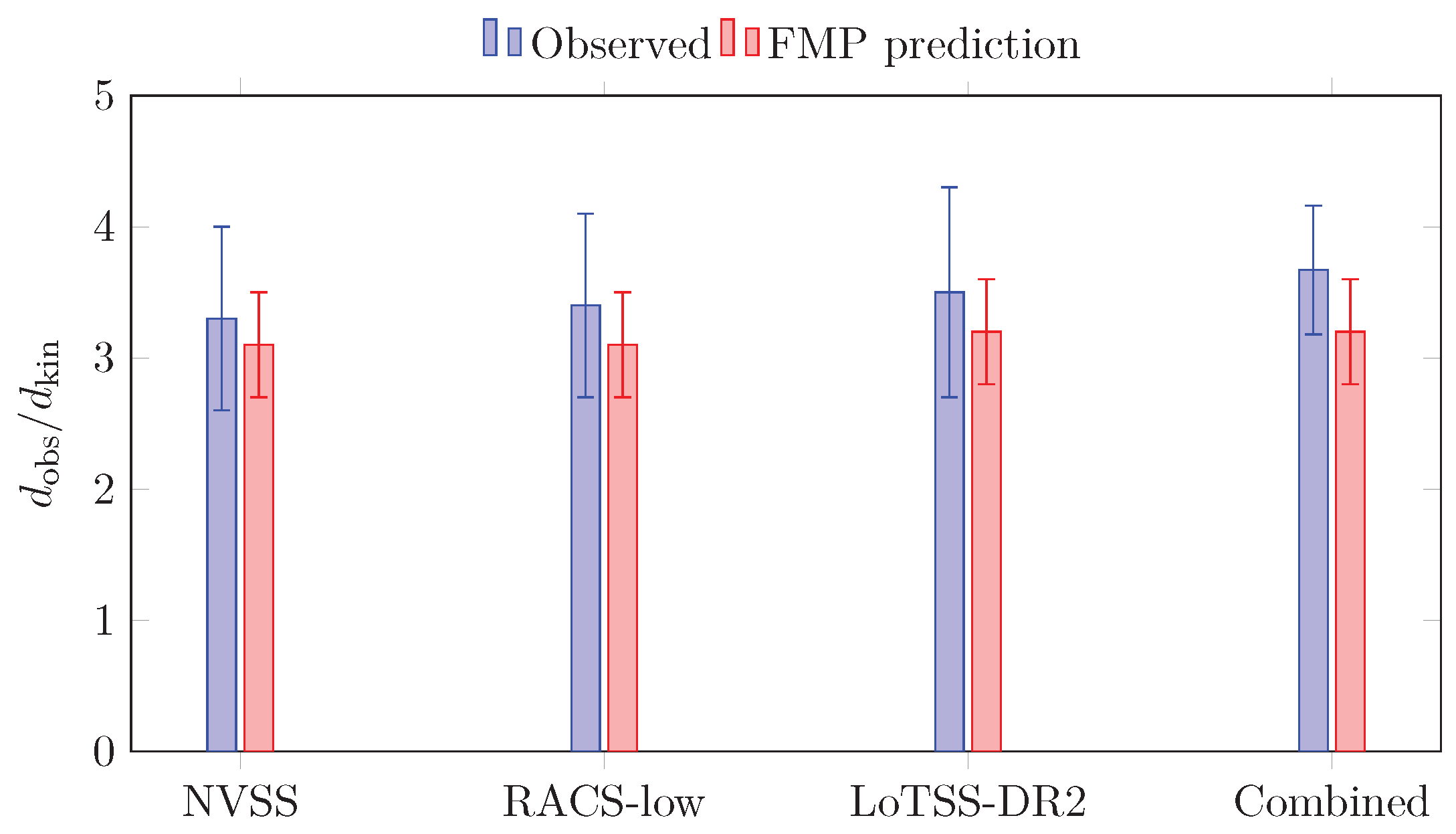

Table 1.
Representative parameters for the selection function and linear bias used for NVSS, RACS–low and LoTSS–DR2 in Eqs. (26) and (27).
| Survey | |||||
|---|---|---|---|---|---|
| NVSS | 1.0 | 1.5 | 0.8 | 1.7 | 0.8 |
| RACS–low | 1.0 | 1.5 | 0.7 | 1.6 | 0.8 |
| LoTSS–DR2 | 1.2 | 1.6 | 0.9 | 1.8 | 0.9 |
Table 2.
Representative ULS boost factors for three kernel realisations consistent with and the absence of ULS effects on galaxy and cluster scales. The quoted uncertainties reflect the spread over reasonable and models as well as the priors on .
Table 2.
Representative ULS boost factors for three kernel realisations consistent with and the absence of ULS effects on galaxy and cluster scales. The quoted uncertainties reflect the spread over reasonable and models as well as the priors on .
| Kernel | (combined) | |||
|---|---|---|---|---|
| A (low ULS) | 0.20 | 0.011 | ||
| B (fiducial) | 0.25 | 0.008 | ||
| C (high ULS) | 0.30 | 0.006 |
Disclaimer/Publisher’s Note: The statements, opinions and data contained in all publications are solely those of the individual author(s) and contributor(s) and not of MDPI and/or the editor(s). MDPI and/or the editor(s) disclaim responsibility for any injury to people or property resulting from any ideas, methods, instructions or products referred to in the content. |
© 2025 by the authors. Licensee MDPI, Basel, Switzerland. This article is an open access article distributed under the terms and conditions of the Creative Commons Attribution (CC BY) license (http://creativecommons.org/licenses/by/4.0/).
Copyright: This open access article is published under a Creative Commons CC BY 4.0 license, which permit the free download, distribution, and reuse, provided that the author and preprint are cited in any reuse.


