
Submitted:
08 December 2025
Posted:
09 December 2025
You are already at the latest version
Abstract
The increasing complexity of smart buildings and the tightening requirements of European regulations have amplified the need for integrated modeling environments capable of assessing automation and control strategies in early design stages. This paper presents a digital-twin-based simulation framework that links building information modeling (BIM) data with MATLAB/Simulink models of heating, ventilation, and air conditioning (HVAC), lighting, and shading systems to support the standardized evaluation of Building Automation and Control Systems (BACS) according to EN ISO 52120 and the Smart Readiness Indicator (SRI). The proposed framework enables rapid scenario development, systematic comparison of automation classes, and assessment of predictive control concepts within a unified, regulation-aligned environment. A representative academic building is used to demonstrate how the toolchain supports consistent simulation of operational states, subsystem interactions, and energy-related behaviors across varying control strategies. The results highlight the ability of the framework to capture performance trends, support compliance-driven decision-making, and provide a basis for the gradual introduction of predictive and artificial intelligence (AI)-enabled methods. The approach offers a structured path to more advanced digital-twin-driven building design, verification, and optimization.

Keywords:
EN ISO 52120
; smart readiness indicator
; building automation and control systems
; digital twin
; building information modeling
; predictive control strategies
1. Introduction
The transition towards a decarbonized and digitalized building sector has led to an increasing focus on intelligent, data-driven energy management. Rather than relying solely on performance indicators in the design-stage, the operational phase of buildings is becoming the primary field for optimization through automation, digital modeling, and predictive control. This evolution reflects the need to integrate physical assets with virtual counterparts capable of simulation, forecasting, and self-adaptation under changing environmental and operational conditions [1,2,3].
In the landscape of European policies, the European Green Deal, the Fit-for-55 Package, and the recast Energy Performance of Buildings Directive (EPBD 2024) establish the foundations for this transformation [4,5]. The directive mandates the broader deployment of Building Automation and Control Systems (BACS) and introduces the Smart Readiness Indicator (SRI) to evaluate the ability of a building to adapt, communicate and optimize its operation [6]. Complementary analyzes by international agencies underscore that digitalization, data exchange, and automation are among the most effective enablers of demand-side flexibility and energy efficiency in buildings [7,8]. The technical basis for this transformation is the convergence of Building Information Modeling (BIM) and the Digital Twin (DT) concept. BIM provides the semantic and geometric description of a building, while DT adds a dynamic layer of simulation, control, and analytics. This combination facilitates the representation of physical systems, including heating, ventilation, air conditioning (HVAC) and lighting within virtual environments capable of real-time prediction, optimization, and decision support [9,10,11,12]. Recent studies further demonstrate the potential of BIM-to-Simulink and co-simulation approaches that connect the physical and control layers for the predictive management of energy performance [13,14,15,16].
However, challenges remain in aligning DT implementations with regulatory and standardized frameworks. While EN ISO 52120 [17] defines detailed classifications and assessment methodologies for BACS energy performance, and the SRI promotes quantitative, data-driven evaluation, only a few simulation tools currently are considered and developed to support both frameworks concurrently [18,19,20]. Commonly used environments such as EnergyPlus, TRNSYS, and IDA ICE have been demonstrated to be efficient for envelope and thermal simulation. However, a limitation of these environments is that they lack interoperability with BIM and do not fully model automation logics. Consequently, the potential for predictive scenario-based evaluation of intelligent control functions remains underutilized [21,22].
To address these limitations, the authors proposed a DT framework, developed in MATLAB/Simulink, and integrated with BIM data. The framework facilitates dynamic simulation of automation scenarios that comply with EN ISO 52120 and SRI guidelines. These scenarios include predictive HVAC control, demand-driven ventilation, and adaptive lighting. It enables the quantification of energy consumption, comfort-related indicators, and control responsiveness, while supporting forecasting under variable operational and external conditions [13,23,24,25].
The contributions of this study are fivefold:
- The development of a regulation-driven DT framework combining BIM and MATLAB/Simulink to model and assess smart building automation according to EN ISO 52120 and SRI;
- Application of the framework for predictive and dynamic evaluation of building energy performance in multiple automation scenarios (HVAC, lighting);
- Introduction of a method for parameterizing automation functions using BIM data and normative guidelines, enabling systematic analysis of trade-offs between energy efficiency, occupant comfort, and system complexity.
- Development of an adaptive control strategy framework that integrates real-time occupancy patterns, environmental conditions, and energy pricing signals to optimize building automation systems, as demonstrated by predictive blind control and dynamic ventilation adjustments in simulation.
- Implementation of a modular simulation environment that enables systematic evaluation of individual SRI functions (e.g., demand response, fault detection) while maintaining system-level interactions, allowing for both component-level optimization and whole-building performance assessment.
This approach provides a toolchain that links geometry and semantics from BIM, control logic from BACS, and predictive capabilities of DTs within regulatory frameworks. The final integration provides a framework for decision-making processes related to the design, retrofit, and operation of buildings that are prepared for the integration of smart-technology systems. These systems are in alignment with the establishment of objectives concerning energy efficiency and sustainability [11,12].
The paper is structured as follows: Section 2 reviews background work on DTs, BIM integration, and regulation-aligned automation assessment. Section 3 introduces the modeling framework and the simulation workflow. Section 4 presents results for the three automation scenarios, and Section 5 provides a comparative discussion. Section 6 concludes the study and describes the direction for future development.
2. Background and Related Work
This section is a continuation of the context presented in Section 1, in which the technological and methodological underpinnings of the digitalization of building operations are examined. The text focuses on the evolution of DT and BIM into core tools for energy simulation and automation analysis. It also examines how regulatory frameworks, such as EN ISO 52120 and the SRI, guide their application. In addition, it explores the current limitations and research opportunities in this field. Consequently, these aspects delineate the foundation for developing and assessing simulation-based approaches to smart, regulation-compliant building performance.
2.1. Integration of Digital Twin and BIM for Smart Buildings
The concept of DT has evolved from static digital models into dynamic, cyber-physical counterparts capable of representing, simulating, and predicting the behavior of real buildings. DTs integrate sensor data, physical models, and control algorithms to replicate system responses under variable boundary conditions and operational contexts [11,26]. In the construction sector of buildings, there is an increasing emphasis on optimizing energy use, indoor environmental quality, and maintenance processes [3,27]. Arowoiya et al. [1] and Buonomano et al. [9] demonstrated that coupling BIM-based geometry with MATLAB/Simulink co-simulation enables dynamic evaluation of HVAC and lighting functions, improving both thermal comfort and control precision. Concurrently, Han et al. [10] and Cespedes-Cubides and Jradi [11] corroborated the efficacy of predictive DT models integrated with AI and edge analytics to predict energy loads and detect inefficiencies before they occur.
A notable example of a holistic approach is DanRETwin, developed at Aalborg University in Denmark [2,28]. The project integrates BIM, sensor networks, and artificial intelligence (AI)-based predictive control for a university building, allowing continuous comparison between simulated and measured data. The DT facilitated adaptive HVAC operation, based on occupancy and weather forecasts, thus reducing heating demand by 15% while maintaining comfortable conditions. This case exemplifies the efficacy of integrating BIM semantics with MATLAB/Simulink and real-time feedback for operational optimi DTand post-occupancy evaluation.
Integration of BIM and DT is a foundational element for further digitalization of smart building. BIM provides the static geometric and semantic structure of building systems, while DT technology adds the dynamic simulation layer that enables forecasting and adaptive control [15]. However, as Deng et al. [29] observed, most BIM implementations remain descriptive, lacking sensor semantics and control information, which limits interoperability with simulation tools. Omrany et al. [30] and Kyriaki et al. [15] further emphasized the importance of consistent data exchange, linking BIM semantics to operational parameters and real-time feedback, for the scalable deployment of DT in buildings.
2.2. Standards and Quantitative Assessment Frameworks (BACS and SRI)
BACS plays a central role in the operational performance of contemporary buildings. The international standard EN ISO 52120 [17] delineates the contributions of automation, control, and technical building management (TBM) to energy efficiency, introducing classes A–D to categorize the level of control sophistication. As demonstrated by Vandenbogaerde et al. [19], Class A systems have been shown to achieve substantial energy savings through the implementation of adaptive HVAC control, daylight-dependent lighting, and coordinated ventilation. The standard also introduces “BACS efficiency factors,” which quantify the expected performance improvements and can be integrated into simulation environments. As demonstrated in [25], the EN ISO 52120 parameters can be implemented directly in MATLAB/Simulink. This enables a quantitative comparison aligned with the regulation of automation strategies.
A representative case is the Austrian Smart Readiness Pilot reported by Märzinger and Österreicher [18]. The project applied SRI and EN ISO 52120 to a mixed-use building district, evaluating load-shifting and control capabilities through simulation. The analysis revealed that predictive control and occupancy-linked ventilation increased the SRI score by 24% compared with baseline scheduling. Similar outcomes were observed in hybrid control studies for Polish public buildings [25], where MATLAB-based modeling confirmed energy savings and functional improvements in compliance with EN ISO 52120.
Currently, the SRI, as outlined in EPBD 2024 [4], offers a standardized framework to evaluate a building’s capacity to respond to user demands, system operations, and grid conditions. The SRI differentiates between qualitative (Methods A, B) and quantitative (Method C) evaluation approaches. The latter necessitates meticulous simulation or monitoring of automation effects. Delavar et al. [12] underscored the need for data-driven simulation-based evaluation to transform the SRI into a practical tool for operational analysis.
To illustrate these relationships, Table 1 provides a summary of selected studies that demonstrate the degree of integration between DT/BIM, compliance with standards, and quantitative assessment capabilities.
2.3. Standards and Quantitative Assessment Frameworks (BACS and SRI)
Despite the significant advances observed in this field, the majority studies address isolated technological or analytical aspects—such as predictive HVAC control, occupant-centric comfort modeling, or AI-based optimization—without establishing links to normative frameworks for consistent performance evaluation [11,12,13,20]. Omrany et al. [30,31] observed that DT implementation remains fragmented and rarely integrates standardized assessment criteria. Concurrently, Kyriaki et al. [15] and Delavar et al. [12] emphasize that SRI Method C, which requires simulation-supported quantification, has been constrained in its practical implementation. The identified research gap thus concerns the absence of integrated regulatory-oriented frameworks that combine BIM semantics, DT simulation, and BACS logic for a systematic and repeatable evaluation of smart readiness.
The authors of this paper aim to explore how simulation-based methods can support and illustrate the evaluation of automation functions according to EN ISO 52120 and SRI. To this end, they have developed a DT framework in MATLAB/Simulink and linked it to BIM data. The objective of this study is to demonstrate the feasibility and potential of this approach as a data-driven complementary tool for a consistent assessment of building smartness and energy performance.
3. Materials and Methods
This section presents the simulation framework developed in MATLAB/Simulink for the performance assessment of BACS and the evaluation of smart-readiness functionalities in accordance with EN ISO 52120 and the SRI methodology. The objective of the proposed framework is to replicate, analyze, and compare intelligent control strategies at different automation maturity levels, corresponding to BACS Class C, Class A, and a high-SRI predictive configuration. This will be achieved using a unified DT environment.
The modeling approach integrates a simplified, BIM-derived building representation with thermal-zone simulation, occupancy modeling, HVAC control, and lighting control subsystems. MATLAB/Simulink was selected as the simulation environment due to its capability to model both physical processes and control logic concurrently. This capability enables the evaluation of automation functions, as opposed to solely thermal behavior, in a regulation-aligned manner. In contrast to conventional building performance tools (e.g., EnergyPlus, TRNSYS, IDA ICE), the proposed framework facilitates the explicit implementation of BACS logic, fault-detection mechanisms, demand-driven strategies, and predictive control algorithms, as specified by SRI Method C. The developed DT model incorporates artificial lighting, occupancy sensors, and HVAC subsystems while supporting scenario-based simulations that explore the interactions between automation functions. This enables a modular and comprehensive evaluation of smart-readiness measures and the quantification of their impact on energy performance, comfort, and operational responsiveness within a controlled simulation environment.
3.1. Reference Building Model and BIM-Derived Spatial Representation
The simulation model represents a concept of academic non-residential buildings designed as a simplified but structurally coherent analog of the building automation laboratories located in the AGH University of Krakow (AutBudNet) [32]. Although the real building served as conceptual inspiration for spatial composition and zoning logic, the model used in this study is not a digital replica of the existing facility. Instead, it constitutes an intentionally abstracted and parametric configuration that preserves realistic architectural proportions, zoning relationships, and occupancy patterns, while allowing full computational control and reproducibility of the simulation.
3.1.1. Spatial Layout and Zoning
The reference building model consists of two identical floors, each with a clear story height of 3 m, resulting in a total modeled height of 6 m. Both floors follow a modular L-shaped plan and are subdivided into five functional thermal zones representative of typical academic-use spaces:
- AutBudNet Lab (main laboratory; 12 m × 8 m);
- Office (4 m × 5 m);
- ITRoom (3 m × 5 m);
- Warehouse (5 m × 3 m);
- FireExit corridor (8 m × 2 m).
The zone arrangement is defined using a Cartesian coordinate system, allowing all spatial relations to be parameterized and programmatically modified. The external walls incorporate window openings with predefined glazing ratios (e.g., 50%, 40%, and 60% for selected orientations), while the internal partitions differ in solidity depending on their structural or fire-safety function.
Figure 1 and Figure 2 illustrate the spatial organization and placement of lighting fixtures used in the simulation model. The BIM-derived geometry was converted into a simplified parametric representation, serving as the basis for thermal zone definitions in Simscape and for assigning building envelope parameters later described in Section 3.4.
3.1.2. Occupancy Modeling
Occupancy plays a critical role in determining internal gains, ventilation demand, and lighting operation. Occupancy schedules were defined to reproduce typical usage patterns of academic laboratory facilities while allowing for scenario-based automation testing:
- AutBudNetLab: follows a fixed weekday schedule (08:00–20:00), representing didactic and project activities, and remains unoccupied during weekends;
- Office: follows a conventional weekday occupancy pattern (08:00–18:00, Monday–Friday), without use on weekends;
- ITRoom: incorporates scheduled access (08:00–18:00) and a 60% random occupancy probability to represent irregular technician visits typical for server and equipment rooms;
- Warehouse: operates daily from 07:00–15:00, modeling shift-based industrial-type use with constant occupancy during work hours;
- FireExit simulates irregular daytime traversal (07:00–19:00) using a 40% random presence probability, reflecting unpredictable transitional use.
The schedules were implemented as time-dependent occupancy vectors with stochastic components, where applicable. These vectors influence internal heat gains, ventilation requirements, and lighting activation, enabling exploration of automation responses across BACS Classes C and A and high-SRI predictive configurations. Figure 3 and Figure 4 (occupancy timelines and cumulative occupancy hours) visualize the temporal distributions applied to two floors. These occupancy assumptions directly influence the operation of the HVAC and lighting control systems and are essential for evaluating automation strategies under the BACS and SRI guidelines.
3.1.3. Nature of the Model
Although inspired by a real AGH infrastructure facility, the building used in this study should be interpreted as a simulation artifact, deliberately designed to provide:
- reproducible and parametric geometry;
- controllable variation of boundary conditions;
- flexible integration with automation scenarios;
- a representative but non-site-specific test environment for BACS and SRI evaluation.
This approach allows DT to serve as a computational benchmark for comparing different automation strategies without the constraints imposed by real-building retrofits, incomplete monitoring data, or uncertain construction parameters.
3.2. HVAC System Model in MATLAB/Simulink with Simscape
Building on the spatial and functional layout of the reference building model, the HVAC subsystem was implemented in MATLAB/Simulink using Simscape libraries. The architecture integrates thermal zoning, air–water heat pump operation, hydraulic flow control, and digital automation logic into a unified simulation framework. This allows both physical behavior and control algorithms to be analyzed concurrently—an essential requirement for evaluating BACS functionalities according to EN ISO 52120 and the quantitative SRI Method C. Figure 5a presents the high-level diagram of the HVAC model, while Figure 5b shows the control subsystem that forms the core of the DT.
The heat pump subsystem is modeled as a closed-loop temperature controller that integrates mode selection with hydraulic flow management. Control is based on the temperature error:
where: – temperature setpoint; – measured room temperature; – instantaneous temperature error.
The error is discretized using the operator to emulate sample-and-hold digital control, producing a preliminary valve command . Valve actuation uses a signed-magnitude scheme: the magnitude is shaped by a continuous PID controller, then recombined with its sign to ensure correct heating or cooling direction. The final command is filtered in discrete time before driving the valve, enabling precise hydraulic modulation.
Hydraulic flow routing is conditional on the operational state . The nominal flow is permitted only when the heat pump is active:
where: – waterflow rate; – nominal design flow; – operation mode (-1 heating, 0 off, +1 cooling).
Operational mode is determined using a dual-threshold hysteresis based on the accumulated temperature error, defined as:
where: – temperature setpoint; – measured room temperature; – instantaneous temperature error.
Cooling () is activated when exceeds the upper threshold, and heating () when it drops below the lower threshold. A deadband prevents rapid toggling near the setpoint. A valve interlock enforces when . An auxiliary electric heater is represented by the signal , which supplies fixed nominal power under extreme load or manual override.
Thermal performance is obtained by interpolation of EN 14511 [33] manufacturer data. Real-time heating/cooling capacity and coefficient of performance (COP) are estimated by matching instantaneous operating conditions to certified test points (e.g., A7W35, A-2W55) using polynomial fits or lookup tables, capturing part-load behavior and temperature-dependent efficiency. On this basis, the model computes the instantaneous thermal power delivered or absorbed by the heat pump, which is subsequently integrated over time to determine the HVAC energy consumption reported in the results section. The heat exchanger model includes coil geometry, internal water volume representing thermal mass, log mean temperature difference LMTD-based heat-transfer calculations and empirically fitted refrigerant-cycle characteristics. The complete set of model outputs consists of the operational state, hydraulic flow, valve position command, and auxiliary heater status. Together, these variables form the control vector used for supervisory integration within BEMS and for evaluating the dynamic response of the heat pump in simulation.
This output vector encapsulates the essential thermal and hydraulic actuation states required to reproduce the operating behavior of the system under varying load and boundary conditions.
3.3. Lighting System Model in MATLAB/Simulink with Simscape
The lighting subsystem is incorporated into the MATLAB/Simulink and Simscape modeling framework to enable the analysis of its impact on building energy performance and smart-control functionality. The model is implemented in several configurations, representing different levels of system complexity and response to environmental conditions and occupancy signals. These variants support the evaluation of selected BACS functions in accordance with EN ISO 52120 and the SRI methodology.
For the baseline simulation scenario, fixed power ratings of luminaires were assigned to selected rooms of the reference building. Each room is represented by an aggregate lighting load, defined as the sum of installed luminaires. To represent total electrical demand in each zone, the lighting load is modeled as follows:
where: – total lighting power assigned to a room; – power rating of luminaire ; – number of luminaires in the room.
The power values adopted are summarized in Table 2 and used during the initial simulation experiments to assess the demand for lighting energy and the interaction of lighting control algorithms with other subsystems of buildings.
The system implements a sophisticated daylight harvesting algorithm that continuously adjusts artificial light output based on real-time solar radiation measurements, maintaining optimal levels of illuminance while minimizing energy consumption. Occupancy-based control is enhanced with randomized operation patterns in shared spaces to prevent the “empty room” effect, where lights turn off immediately after occupants leave, improving both energy efficiency and user experience. The lighting model includes a configurable time-step resolution (defaulting to 15-minute intervals) to accurately capture the dynamic interaction between natural light availability and artificial lighting demand throughout the day. A fault detection mechanism is integrated to identify abnormal power consumption patterns, alerting facility managers to potential equipment malfunctions or maintenance needs in the lighting system. The system’s control logic features adaptive dimming curves that account for room orientation and window characteristics, with specific transmittance coefficients (40-60% range) applied to different window walls to optimize daylight utilization.
3.4. General Assumptions and Conditions for the Model
The energy model for the building was adapted to the Polish climatic conditions and national construction standards. The thermal parameters were recalibrated to reflect local insulation requirements, heating-season demands, and required U-values for opaque and transparent envelope elements. The reference building was placed in a representative urban location in Warsaw, and regional weather data and solar calculations were applied to capture seasonal variations in solar gains and heat losses.
The lighting subsystem was extended with an occupancy-responsive control strategy that corresponds to Polish work schedules, room-specific occupancy profiles, daylight availability, and task-related illumination needs. Its integration with the thermal model enables a coherent representation of electrical lighting loads and the resulting internal heat gains, thereby improving the accuracy of energy-flow predictions for Central European contexts. All modifications maintain complete compatibility with the original HVAC and thermal-zone structure. The calibrated L-shaped geometry, the thermal-network configuration and the fenestration layout were preserved. The updated model provides more reliable annual energy estimates by incorporating Poland’s characteristic climate, defined by cold winters and mild summers, and typical building operation patterns.
The core features for HVAC assessment, envelope performance evaluation and energy-efficiency analysis remain available and are complemented by new lighting-optimization capabilities. These region-specific enhancements increase the applicability of the model to Polish regulatory compliance, retrofit scenario development, and academic research. The adapted model supports robust evaluation of seasonal energy use, peak-demand behavior, and interactions among lighting, occupancy, and HVAC systems.
4. Results
Building on the modeling framework established in Section 3, the simulation phase aims to verify the behavior of the DT model developed under different levels of building automation. To evaluate the impact of BACS and SRI-related control strategies on functionality, the authors assessed the model using three representative scenarios: a baseline BACS Class C configuration, an advanced Class A configuration, and a high-SRI predictive setup. The reference building geometry, thermal-zone structure, occupancy patterns, and climatic boundary conditions remained unchanged across all scenarios, ensuring that any observed performance differences were solely the result of the applied automation strategies.
The results reported in this section correspond to the complete two-floor model and were obtained from a consistent 24-hour simulation period, using the same seasonal weather data set for Warsaw and synchronized occupancy schedules. The analysis focuses on the electricity use of the HVAC and lighting subsystems, the total energy demand, and the zone-level consumption profiles. This is complemented by qualitative observations on control responsiveness and interactions between lighting, shading, and thermal loads. This combined set of indicators enables an evaluation of automation performance that is in accordance with EN ISO 52120 and the SRI.
4.1. Scenario A – Baseline Class C Operation
Scenario A represents the baseline configuration corresponding to BACS Class C from EN ISO 52120, which is used as a reference point to evaluate the enhancements introduced in more advanced automation setups. This scenario implements simple, independent control strategies for heating, ventilation, and lighting without any inter-system coordination or predictive behavior. All control functions operate in a deterministic manner, driven solely by fixed setpoints and binary occupancy signals. This scenario reflects the typical low-complexity installations found in older or minimally automated non-residential buildings. Heating is regulated using a constant set point of 17 °C with individual control at room-level. Although cooling is technically enabled, it is rarely activated due to the low setpoint and climatic conditions. Ventilation operates as a fixed-airflow system that is turned on when occupancy is detected, without demand modulation. Lighting follows an on/off strategy using occupancy sensors and manual switches with no daylight-related dimming. Blinds are operated only manually and do not affect thermal or lighting loads. Table 3 summarizes the main operational characteristics of Scenario A.
The 24-hour simulation of the two-story model yields a total energy consumption of 12.85 kWh, with lighting representing the dominant share of the load. The HVAC subsystem contributes 38.5%, while lighting accounts for 61.5% of total energy use. Table 4 presents the subsystem-level energy balance.
A zone-level breakdown confirms the significant influence of operational schedules and room size. The AutBudNet Lab shows the highest daily demand due to its extended occupancy period and the highest installed lighting power. Smaller rooms such as the IT Room or Office exhibit proportionally lower consumption. Detailed values are shown in Table 5.
The results indicate that the absence of daylight harvesting and adaptive lighting control is the main cause of the high demand for lighting energy. Artificial lighting operates at full power during all occupied hours, regardless of available daylight. HVAC energy use remains moderate due to the low heating setpoint; however, the fixed-airflow ventilation strategy introduces inefficiencies, as airflow does not adjust to actual occupancy or indoor air quality conditions. The energy 24 hour profiles for the use of HVAC energy in all rooms are presented in Figure 6.
The HVAC power and temperature profiles presented in Figure 7 demonstrate the limited dynamic behavior of the Class C control logic. Heating demand remains low, with short pulses of thermal power maintaining the fixed set point of 17 °C throughout the day. No cooling activation is observed, which is consistent with the applied climatic conditions and low setpoint definition. Ventilation operates uniformly during occupancy periods, resulting in a steady baseline power load due to the fixed-airflow strategy. The temperature curves remain close to the setpoint, indicating stable but non-adaptive control performance.
In addition, the lighting operation profile for Scenario A is illustrated in Figure 8, which shows continuous activation of the luminaires during all scheduled occupancy periods. The characteristic step-like trajectories reflect the binary on/off control strategy and the absence of daylight-responsive dimming. Zones with extended occupancy—particularly the AutBudNet Lab and the Office—exhibit long intervals of uninterrupted lighting operation, while transition spaces such as the FireExit corridor display shorter and irregular activation patterns corresponding to stochastic use. The figure confirms that lighting operates at full installed power whenever a zone is occupied, directly contributing to the high overall lighting energy demand.
In general, Scenario A establishes a clear baseline for future analysis. Highlights the limitations of simple Class C automation and identifies lighting control as the subsystem with the highest potential for meaningful energy savings in more advanced configurations.
4.2. Scenario B – Advanced Class A Operation
Scenario B represents an advanced automation configuration that is aligned with BACS Class A from EN ISO 52120. In contrast to the simple, independent controls of Scenario A, this setup introduces coordinated, adaptive, and partly predictive strategies. Key functions include occupancy-proportional ventilation, daylight-responsive lighting control (dimming), heat recovery, and free or pre-cooling under favorable outdoor conditions. Although the thermal, spatial, and occupancy assumptions remain unchanged, enhanced control capabilities allow for more responsive operation and significantly reduced energy demand [34].
The heating system uses an adaptive 0.5 °C deadband to enable more precise temperature control. Ventilation uses demand-controlled airflow, which adjusts the fan operation according to occupancy levels. The intensity of the light is continuously modulated according to the availability of daylight, particularly in rooms facing south. Solar protection is analyzed in two variants: one with automated blinds that respond to solar gains and one without blinds, assuming no shading control. This configuration allows for the assessment of shading as an interacting subsystem. Table 6 summarizes the main operational characteristics of Scenario B.
Scenario B was evaluated in two variants — with and without automated blinds — to isolate the influence of shading control. In both cases, the total energy demand was substantially lower than the baseline for Scenario A (12.85 kWh). For the automated blind configuration, consumption decreased to 6.52 kWh, representing a savings of almost 50%. Lighting energy use drops markedly due to continuous daylight-responsive dimming, while HVAC demand is reduced through heat recovery, free cooling and demand-controlled ventilation. The subsystem-level results for both variants are summarized in Table 7.
The introduction of automated blinds results in a slight increase in the use of HVAC electricity (0.031 kWh). Although shading reduces solar gains, it can also require additional heating or ventilation to maintain comfort conditions. Lighting consumption remains unchanged, as daylight dimming fully compensates for reduced natural light. This interaction between shading and HVAC illustrates the complexity of multi-system optimization characteristic of Class A automation.
The room-level results summarized in Table 8 clearly illustrate the impact of the advanced control functions introduced in Scenario B.
Lighting demand decreases in all zones due to continuous daylight-aware dimming, which limits artificial lighting whenever natural illumination is available. HVAC consumption is likewise reduced, driven by demand-controlled ventilation that lowers airflow during partial occupancy, as well as by heat-recovery and free-cooling strategies that reduce mechanical heating and cooling effort. Automated blinds further stabilize thermal loads by moderating solar gains, supporting reduced cooling demand and contributing to a more balanced temperature profile. Together, these coordinated mechanisms result in noticeably lower total energy use in all rooms analyzed, confirming the effectiveness of Class A automation in improving operational efficiency.
By modifying solar gains, shading alters the amount of heating and ventilation required to maintain the target temperature. This contributes to reducing the demand for HVAC, in conjunction with the improvements introduced by Class A control strategies. These reductions — from 4,95 kWh to 2,27 kWh — result from demand-controlled ventilation in response to occupancy, as well as free cooling and pre-cooling, which limit the need for mechanical cooling. Heat recovery further improves the system’s coefficient of performance (COP). These mechanisms generate markedly lower overall HVAC energy profiles for rooms, as shown in Figure 9.
The HVAC power and temperature profiles shown in Figure 10 reflect the more dynamic behavior of the Class A control strategy.
In contrast to the stable but non-adaptive operation observed in Scenario A, heating and ventilation respond continuously to occupancy signals and varying thermal loads. Demand-controlled ventilation reduces fan power during partial use of the rooms, while heat-recovery and free-cooling events contribute to lower mechanical heating and cooling demand. The temperature curves remain close to the comfort band but exhibit smoother and more frequent adjustments due to the tighter 0.5 °C deadband. A slight increase in HVAC electricity use is visible in the variant with automated blinds, resulting from the additional heating or ventilation effort required to compensate for the reduced solar gains. This minor increase reflects the interplay of shading and demand-controlled ventilation (DCV) functions, where actions that limit overheating may introduce small thermal compensation loads. In general, the profiles confirm that Scenario B achieves higher responsiveness and improved energy efficiency while maintaining stable indoor temperatures under advanced Class A automation [35].
Next, Figure 8 shows the patterns that demonstrate a pronounced reduction in lighting energy, where artificial lighting is continuously dimmed in response to available daylight throughout the day. South-facing rooms benefit the most from natural light, substantially reducing the required electric lighting output, while zones that are used intermittently contribute additional savings due to shorter activation periods. It is notable that lighting consumption remains identical in both blind sub-scenarios, indicating that the daylight-aware dimming algorithm fully compensates for the reduced daylight caused by shading. This confirms that the control system maintains the target illuminance level without generating additional electrical demand, making lighting one of the most effective contributors to overall energy reduction in Scenario B.
Taking into account all the issues discussed, scenario B provides an intermediate performance benchmark between the baseline and the fully predictive configuration analyzed further in Scenario C.
4.3. Scenario C – High SRI with Predictive Operation
Scenario C represents the most advanced configuration in this study, aligned with a high SRI level [6]. Expanding on the adaptive Class A automation of Scenario B, it integrates predictive control, real-time optimization, and weather-based forecasting through model predictive control (MPC). With unchanged physical, thermal, and occupancy assumptions, Scenario C provides a fully comparable, yet higher-performance benchmark driven by forecasting, proactive shading, and advanced ventilation control [36,37].
Heating and cooling use predictive setpoint optimization, enabling earlier free-cooling or pre-cooling. Ventilation adjusts airflow dynamically beyond simple occupancy-based logic. Lighting employs adaptive scenes that continuously modulate the illuminance according to daylight and task needs. Predictive blind control anticipates solar gains and proactively adjusts shading. The main control characteristics of Scenario C are summarized in Table 9. The SRI assessment of the automated building automation systems implemented, excluding the Hot Water (DHW) and Electric Vehicle (EV) charging infrastructure (not considered in this approach model), yields a score of 91.7%, reflecting advanced HVAC, lighting, and shading control capabilities that significantly enhance energy efficiency, occupant comfort, and grid responsiveness.
Scenario C achieves the lowest total energy consumption of all the scenarios discussed. Predictive control further reduces lighting energy significantly, while HVAC consumption is a little higher than for Scenario B. Nevertheless, an analysis of the final results indicates that the overall energy consumption for lightning and HVAC with blind control is lower in this scenario C compared to the previous ones. Subsystem-level results for variants with and without the active blinds control are presented in Table 10.
It is clear that the lighting consumption remains unchanged in both variants. The advanced dimming algorithm fully compensates for the reduced daylight caused by blind activation, maintaining the target illuminance through smooth modulation of artificial lighting [38]. Consequently, HVAC is the only subsystem that benefits from predictive shading, confirming the structural decoupling between lighting and blinds in Scenario C.
Room-level results also confirm the advantages of fully integrated predictive control. All zones experience reduced total energy usage compared to Scenario B, with the most significant gains observed in rooms oriented toward the south due to proactive shading and improved thermal stability. Table 11 summarizes the energy consumption per-room for Scenario C with blinds.
The energy consumption of HVAC in Scenario C is slightly higher than in Scenario B (increasing from 2.27 to 2.59 kWh with blinds). This rise is associated with the more stringent environmental control applied in the predictive configuration, which requires frequent airflow adjustments to maintain stable indoor conditions. The advanced control logic responds more dynamically than the occupancy-based approach in Scenario B, resulting in a marginal increase in fan and ventilation effort. At the same time, the use of MPC ensures that these adjustments are optimized with respect to energy use and comfort constraints, balancing thermal stability with operational efficiency. These effects are reflected in the 24-hour power and temperature trajectories shown in Figure 12, which demonstrate the more responsive behavior of the HVAC subsystem under predictive high-SRI operation.
The HVAC power and temperature trajectories in Figure 13 demonstrate increased responsiveness compared to Scenario B. MPC enables smoother temperature curves and earlier activation of cooling or ventilative strategies based on forecasted conditions. Indoor Air Quality (IAQ)-driven DCV results in more frequent airflow adjustments, which explains the small increase in HVAC energy relative to Scenario B. This increase is due to tighter IAQ requirements and higher airflow rates triggered by pollutant sensors, reflecting a trade-off between energy efficiency and indoor environmental quality [38].
In addition, predictive blind control produces a clearly visible reduction in cooling-related demand. Unlike in Scenario B, where blinds introduced a minor HVAC penalty due to reactive shading, the forecast-based strategy reduces HVAC effort and improves thermal stability by counteracting solar gains before they occur.
The lighting operation profiles for Scenario C (Figure 14) show a more pronounced modulation than in Scenario B. The adaptive lighting scenes continuously adjust the illuminance, reflecting both daylight availability and task requirements. The system achieves the lowest lighting energy of all scenarios (3.60 kWh), a reduction of almost 15% compared with Scenario B. The profiles confirm that lighting behavior is fully decoupled from shading: blind operation does not increase lighting demand due to the advanced dimming algorithm’s ability to maintain target illuminance without additional energy.
Scenario C provides the lowest total energy consumption across all operational configurations and demonstrates the strongest synergy between predictive shading, IAQ-based ventilation, and task-adaptive lighting control. Overall, Scenario C establishes the highest performance benchmark, demonstrating that predictive, sensor-rich, and fully integrated BACS can optimize both energy efficiency and indoor environmental quality within a unified Smart Readiness–aligned framework.
5. Comparison and Discussion
Building on the detailed quantitative results presented in Section 4, this section synthesizes the main performance differences observed across the three automation scenarios and interprets them from the perspective of smart-readiness, system integration, and operational efficiency. The comparative discussion highlights the progression from basic to predictive control and provides the analytical context necessary for longer-term assessments introduced in the subsequent weekly analysis.
5.1. Comparative Analysis of Scenarios A, B and C
The comparative analysis of total energy consumption across the three automation strategies, as illustrated in Figure 15 (a), reveals a clear and substantial reduction when transitioning from the baseline Class C configuration to the more advanced Class A operation. This finding provides robust evidence for the significant impact of EN ISO 52120-aligned control functions, particularly daylight dimming, demand-controlled ventilation, and coordinated HVAC logic, on the overall energy performance of buildings. The enhancement observed in Scenario B signifies the most substantial step-change across all comparisons. In contrast, the additional enhancement provided by the high-SRI predictive configuration is discernibly less pronounced, indicating that once Class A automation is established, subsequent gains become incremental and progressively dependent on refined control interactions rather than extensive functional transformations.
A more detailed comparison of the performance at the subsystem-level, as demonstrated in Figure 15 (b), highlights that improvements in efficiency in HVAC and lighting are more nuanced and sensitive to specific application conditions. It is evident that a transition from Scenario A to Scenario B is advantageous for both subsystems. However, the transition to Scenario C no longer results in equivalent gains. The findings reveal that the performance of HVAC systems is influenced by the interplay between predictive control, ventilation requirements, and shading strategies [36,37]. These interactions can generate slight compensatory energy effects that partially offset the benefits of predictive optimization. Despite the fact that lighting performance remains highly efficient, marginal improvements are becoming increasingly negligible as a result of the substantial effectiveness of daylight-aware dimming that has already been implemented in Scenario B. Nevertheless, for the building model and control assumptions analyzed, the combined HVAC and lighting results in Scenario C still exhibit a small but consistent overall reduction relative to Scenario B. This indicates that predictive control—although characterized by more complex interdependencies—can refine system operation in a way that incrementally improves energy efficiency without compromising comfort or indoor environmental quality.
The observed differences in daily energy performance have also provided a foundation for examining multi-day and weekly operation. As the simulation horizon has been extended, the trends identified in the daily analysis have become more pronounced, particularly the cumulative benefits of predictive ventilation and optimized shading. These aspects have been further evaluated in the extended weekly comparison, which has assessed the persistence and scalability of control strategies over longer operational periods.
5.2. Weekly Comparison
Following detailed analysis of 24-hour performance, the weekly (7-day) energy consumption profile offers a crucial perspective on long-term operational stability and the cumulative impact of scheduling across the different scenarios. The weekly totals, summarized in Table 12, represent the sum of energy consumed on a low-demand Sunday through the end of the full cycle. This aggregation inherently dampens the effect of high-demand peak events observed daily, instead reflecting the average efficiency achieved across varying internal and external conditions, including critical low-occupancy weekend periods.
The substantial savings observed daily (approx 50%) translate into robust, sustained weekly savings of approximately 37% for both the Class A and High SRI scenarios. This consistency affirms the enduring effectiveness of both advanced systems (Class A) and envelope improvements (High SRI) regardless of daily fluctuations [38]. While both HVAC and Lighting loads are reduced, the weekly HVAC consumption shows the largest absolute difference between the Class C baseline 39.54 kWh and the advanced scenarios 21. kWh. This underscores that improvements in thermal efficiency—whether through better equipment or passive solar control —are the primary drivers of overall weekly energy reduction. Unlike the Class C baseline, where the weekly HVAC consumption showed a non-linear increase (due to thermal recovery costs), the advanced scenarios exhibit more predictable, stable energy usage across the week. This suggests that the advanced controls in Class A and the improved thermal inertia provided by the High SRI envelope are more effective at mitigating the thermal recovery penalty associated with intermittent weekend operation.
The subsequent subsections break down these weekly totals by scenario, revealing the specific system efficiencies and control strategies that contribute to the reported 37% savings. Figure 16 illustrates the comparison of energy consumption across all scenarios, presenting both 24-hour and weekly results with a breakdown into HVAC and lighting components.
5.2.1. Scenario A – Discussion
The energy-use profile observed for Scenario A (Class C control) shows clear non-linearity between the 24-hour and 7-day results. The weekly total of 75.92 kWh is markedly lower than the linear projection of 89.95 kWh (−15.6%), reflecting the dominant influence of scheduling and occupancy patterns rather than uniform daily repetition. Lighting is the main source of this negative deviation: its weekly use is 34.2% lower than expected because the control logic activates luminaires only during weekday working hours (08:00–18:00). The 24-hour reference day represents a typical weekday, whereas the weekly total includes two weekend days with zero lighting demand. Consequently, the 7-day energy sum cannot be approximated by simple multiplication of the daily baseline.
In contrast, the HVAC load shows a positive weekly deviation of +14.1%, indicating that average heating demand across the full week exceeds that of the representative day. This is a direct effect of the simplified 17 °C temperature control and occupancy-based on/off ventilation. During the weekend, the absence of occupancy eliminates internal gains and ventilation, allowing the building to cool toward outdoor conditions. When activity resumes on Monday, simultaneous occupancy and ventilation rapidly introduce cold outdoor air, increasing the heating requirement needed to restore the 17 °C setpoint. This thermal recovery penalty raises total HVAC energy compared with mid-week steady-state operation.
Overall, Scenario A illustrates how basic, non-optimized scheduling reduces lighting consumption effectively but imposes a compensatory penalty on HVAC performance. The absence of predictive pre-heating or optimized setback strategies results in higher transient loads at the start of the week, reinforcing the inherently non-linear weekly energy profile.
5.2.2. Scenario B – Discussion
Scenario B (Class A) demonstrates a markedly optimized energy profile, driven by advanced control strategies that reduce both absolute consumption and the non-linearity present in the baseline Class C case. The weekly total scales almost perfectly from the daily value, showing only a +3.74% deviation from a simple seven-day extrapolation—an outcome of clear importance in performance assessment. This minimal deviation indicates that the BMS effectively compensates for weekday–weekend scheduling differences and suppresses the transient loads that were prominent in the simpler Class C configuration. Maintaining such near linearity despite varying occupancy schedules and environmental conditions confirms that the integrated Class A controls sustain a stable and optimized operational regime across the full week. The small positive deviation reflects a modest but intentional increase in daily energy use associated with proactive thermal and pre-conditioning strategies.
Weekly lighting consumption shows a significant negative deviation of −13.48%, meaning that cumulative use is substantially lower than the linear daily projection. This non-linearity results directly from the dual lighting strategy combining occupancy detection and daylight-aware dimming. Because most zones—especially offices and laboratories—are fully occupied only Monday to Friday, the effective lighting demand over the 7-day period is inherently reduced. With illuminance continuously adjusted to available daylight, the system supplies artificial lighting only when necessary. The negative deviation therefore reflects the combined effect of limited weekend occupancy and sufficient daylight contribution, both of which reduce the total lighting operating time and intensity compared to a hypothetical full week of high-occupancy, high-demand conditions.
The HVAC load exhibits the strongest non-linearity, with weekly consumption exceeding the linear daily projection by 35.73%. This positive deviation reflects the proactive operation of the Class A system rather than inefficiency. Aggressive thermal pre-conditioning—such as nighttime free-cooling and dawn pre-cooling—requires fan and pump energy during unoccupied hours to reduce peak loads during occupancy, raising the total weekly energy use, especially when these actions continue through the weekend in preparation for the upcoming workdays. Unlike the Class C scenario, energy is not spent reactively in a large Monday morning recovery pulse. Instead, consumption is shifted to low-tariff periods to stabilize indoor conditions, yielding lower power peaks and improved comfort. When aggregated over the full week, however, this systematic anticipatory effort naturally results in a higher total than suggested by a single-day baseline. The notable weekly saving from Automatic Blind Control (1.137 kWh, 5%) further demonstrates the importance of managing solar gains, preventing overheating and avoiding even greater HVAC demand for cooling and ventilation offsets.
The general near-linear energy scaling in Scenario B confirms the success of the integrated BMS in achieving a predictable, high-performance operational standard. The high positive HVAC deviation is interpreted not as inefficiency, but as the cumulative cost of sophisticated pre-conditioning and thermal stabilization strategies, which successfully offset scheduling and thermal recovery effects to achieve high overall efficiency and thermal comfort.
5.2.3. Scenario C – Discussion
Scenario C represents the highest level of smart readiness, integrating predictive management, forecasting, and grid-responsive operation across all building systems. Such an advanced control yields a highly stable and efficient energy profile. The total weekly consumption shows a modest positive deviation of +9.74% from the linear daily projection—higher than in the Class A case, yet still tightly controlled. This increase does not stem from scheduling limitations or thermal recovery effects, but from the continuous, intentional energy expenditure required to operate high-SRI functions, particularly predictive and demand-driven mechanisms. Considering the efficient envelope and the coordinated operation of elements such as predictive blinds and local demand ventilation, most of the observed energy use reflects active climate management rather than compensation for thermal inertia.
The lighting subsystem achieves a remarkable nearly perfect linear scaling with a deviation of only +0.63%. This result highlights the supreme effectiveness of the Class C lighting strategy. The system uses automatic dimming with time-based, adaptive lighting scenes, which adjusts light output not just based on daylight, but also on task and user needs. The almost zero deviation indicates that the average power draw over the full 7-day period is nearly identical to the power draw of the single reference day. This means the system successfully minimizes artificial lighting consumption during low-occupancy weekend periods while efficiently utilizing daylight to dim the load during occupied weekdays, averaging out the consumption with high precision.
The HVAC load shows a substantial positive deviation of +22.39%. Similar to Scenario B, this increase reflects the energy cost of advanced proactive control, but here it is amplified by grid-integration mechanisms. Forecasting, predictive management, and MPC require the system to consume energy in advance—through pre-cooling or pre-heating initiated on the basis of weather and load forecasts. By distributing this anticipatory operation across the week to support comfort and load shifting, the total weekly energy use naturally exceeds what a reactive, single-day measurement would suggest. Dynamic grid-responsive sequencing and DSM signals also contribute during expected grid peaks, the system may pre-cool the building beforehand, shifting demand to off-peak hours. Although advantageous for grid stability, these actions still generate additional energy use, explaining the positive deviation. Predictive Blind Control delivers a notable HVAC saving of 14.1% per day—higher than in the Class A configuration. This improvement reflects the enhanced forecasting accuracy in the high-SRI system, enabling blinds to be adjusted earlier and more precisely to limit solar gains and reduce peak cooling demand.
Scenario C demonstrates a high level of predictive stability, reflected in the near-linear weekly Lighting load. Positive deviations in total and HVAC consumption represent the inherent energy cost of operating a fully predictive grid-integrated system that prioritizes not only efficiency, but also thermal comfort through individual zone control and CO₂/VOC-based ventilation, as well as grid responsiveness. These overheads are integral to maintaining the advanced performance expected in a high-SRI environment.
5.3. Simulation Challenges and Limitations
The MATLAB-based building energy simulation script implements a simplified thermal model with several inherent limitations in its representation of building physics. The thermal dynamics are approximated using a first-order model that linearly updates zone temperatures based on heating/cooling power inputs, without accounting for the full thermal mass effects of building structures. This simplification leads to faster computation but reduces the accuracy of transient thermal behavior predictions.
The lighting control system operates on fixed schedules and basic occupancy patterns, lacking sophisticated daylight harvesting algorithms that would require detailed modeling of light distribution within spaces. The blind control mechanism uses a simplified solar model that estimates irradiance based on time of day and window orientation but does not incorporate actual solar position calculations or account for external shading effects.
The simulation effectively models basic energy consumption patterns across different building zones, with distinct operational profiles for weekdays and weekends. It successfully demonstrates the interaction between HVAC systems and thermal loads of the building, although with simplified heat transfer coefficients. The implementation includes a basic demand response capability that can adjust setpoints based on external signals.
Key technical constraints include the absence of indoor air quality modeling, particularly CO2 and humidity dynamics, which are critical for comprehensive building performance assessment. Control strategies rely primarily on rule-based approaches rather than advanced control algorithms. The simulation architecture is designed for a specific building layout, limiting its flexibility for different configurations without substantial code modifications.
The strength of the model lies in its computational efficiency and ability to provide reasonable energy use estimates, making it suitable for preliminary analysis despite its simplifications in thermal and control system modeling.
The limitations, simplifications, and features of the models described in the paper, as well as the challenges they present, constitute an opening for further research and development work. An outline of this work is presented in the conclusions.
6. Conclusions
This paper demonstrates that the proposed DT framework—combining BIM-derived spatial data with MATLAB/Simulink models of HVAC, lighting, and shading—is a viable and effective environment for regulation-oriented analysis of intelligent building functions. The framework enables systematic implementation of BACS logic in accordance with EN ISO 52120 and supports scenario-based examination of SRI-related functionalities. Its modular structure allows building geometry, control strategies, and operational assumptions to be varied while maintaining full reproducibility, making the platform suitable for iterative development and exploratory research.
The simulations demonstrate that even simplified physical and control models can provide meaningful illustrations of the operational behavior of automation functions and their interactions. This is particularly valuable at the early research and prototyping stages, where computational efficiency, transparency of model structure, and controllability of parameters are essential. Furthermore, the proposed framework establishes a methodological foundation for the authors’ broader concept, with the aim of efficiently leveraging design data, BIM semantics, and digital twins to accelerate the selection, validation, and verification of control, monitoring, and comfort-related functions in buildings. In its mature form, the approach is intended to support fast and regulation-aligned evaluation workflows compliant with EN ISO 52120 classifications and the SRI methodology. This enables a structured comparison of automation capabilities already at the design and pre-deployment stages.
Although there are several limitations, such as reduced thermal-mass representation, simplified solar and IAQ modeling, and rule-based control, the framework has already achieved its intended purpose, which is to enable rapid evaluation of automation concepts, validation of control logic, and support for the design of comparative experiments. These results provide a solid foundation for future research, which will concentrate on extending the DT with more detailed thermal modeling, advanced solar geometry, improved IAQ dynamics, and predictive or data-driven control methods. The enhancements planned for implementation also include the integration of full SRI Method C quantification, predictive diagnostics, and edge-based real-time analytics. These elements align directly with the doctoral research of the first author, thereby advancing the framework toward a comprehensive environment for robust, regulation-aligned smart-building design and assessment.
Author Contributions
Conceptualization, A.O. and G.W.; methodology, G.W.; validation, A.O.; formal analysis, G.W.; investigation, G.W.; resources, G.W. and A.O.; data curation, G.W.; writing—original draft preparation, G.W.; writing—review and editing, A.O.
Funding
This research received no external funding.
Data Availability Statement
Details of the model scripts and datasets related to their parameterization are available from the authors upon request.
Acknowledgments
During the preparation of this manuscript, the author used assistive tools ChatGPT 5.1 and SCOPUS-AI for the purpose of synthesizing the literature. In addition, the Open Writefull tool was used to verify the grammatical and stylistic correctness of the text.
Conflicts of Interest
The authors declare no conflicts of interest
Abbreviations
The following abbreviations are used in this manuscript:
| AI | Artificial Intelligence |
| BACS | Building Automation and Control Systems |
| BIM | Building Information Modeling |
| COP | Coefficient of Performance |
| DCV | Demand-Controlled Ventilation |
| DHW | Domestic Hot Water |
| DSM | Demand-Side Management |
| DT | Digital Twin |
| EPBD | Energy Performance of Buildings Directive |
| EV | Electric Vehicle |
| HVAC | Heating, Ventilation, and Air Conditioning |
| IAQ | Indoor Air Quality |
| MPC | Model Predictive Control |
| SRI | Smart Readiness Indicator |
| VOC | Volatile Organic Compounds |
References
- Arowoiya, V.A.; Moehler, R.C.; Fang, Y. Digital Twin Technology for Thermal Comfort and Energy Efficiency in Buildings: A State-of-the-Art and Future Directions. Energy and Built Environment 2024, 5, 641–656. [Google Scholar] [CrossRef]
- Jradi, M.; Madsen, B.E.; Kaiser, J.H. DanRETwin: A Digital Twin Solution for Optimal Energy Retrofit Decision-Making and Decarbonization of the Danish Building Stock. Applied Sciences 2023, 13, 9778. [Google Scholar] [CrossRef]
- Bjørnskov, J.; Jradi, M. An Ontology-Based Innovative Energy Modeling Framework for Scalable and Adaptable Building Digital Twins. Energy Build 2023, 292, 113146. [Google Scholar] [CrossRef]
- European Parliament Directive (EU) 2024/1275 of the European Parliament and the Council on the Energy Performance of Buildings; EU: Strasbourg, France, 2024.
- European Commission; European Parliament. European Economic and Social Committee State of the Energy Union Report 2023; Brussels, 2023. [Google Scholar]
- Stijin, Verbeke; Dorien, Aerts; Glenn, Reynders; Yixiao, Ma; Paul, Waide. FINAL REPORT ON THE TECHNICAL SUPPORT TO THE DEVELOPMENT OF A SMART READINESS INDICATOR FOR BUILDINGS; Brussels, 2020. [Google Scholar]
- International Energy Agency; I. Energy Efficiency 2024 2024.
- International Energy Agency; I. Using Digitalisation in Emerging Markets and Developing Economies to Enable Demand Response in Buildings; 2023. [Google Scholar]
- Buonomano, A.; Forzano, C.; Giuzio, G.F.; Palombo, A.; Salzano, A.; Russo, G. Optimizing Building Performance: A Novel Digital Twin Framework for Enhanced Thermal Comfort. In Proceedings of the 2024 3rd International Conference on Energy Transition in the Mediterranean Area (SyNERGY MED), October 21 2024; IEEE, 2024; pp. 1–5. [Google Scholar]
- Han, F.; Du, F.; Jiao, S.; Zou, K. Predictive Analysis of a Building’s Power Consumption Based on Digital Twin Platforms. Energies (Basel) 2024, 17, 3692. [Google Scholar] [CrossRef]
- Cespedes-Cubides, A.S.; Jradi, M. A Review of Building Digital Twins to Improve Energy Efficiency in the Building Operational Stage. Energy Informatics 2024, 7, 11. [Google Scholar] [CrossRef]
- Delavar, T.; Borgentorp, E.; Junnila, S. The Smart Buildings Revolution: A Comprehensive Review of the Smart Readiness Indicator Literature. Applied Sciences 2025, 15, 1808. [Google Scholar] [CrossRef]
- Turco, L.; Zhao, J.; Xu, Y.; Tsourdos, A. A Study on Co-Simulation Digital Twin with MATLAB and AirSim for Future Advanced Air Mobility. In Proceedings of the 2024 IEEE Aerospace Conference; IEEE, March 2 2024; 2024; pp. 1–18. [Google Scholar]
- Kotaru, S.D.; Tandel, Kartik S; Rammohan, B; Babu, Kamal. Integrating Python and MATLAB for Digital Twin Applications in Aeroservoelasticity. Acceleron Aerospace Journal 2025, 4, 872–885. [Google Scholar] [CrossRef]
- Kyriaki, E.; Giama, E.; Theodoridou, I. Machine Learning, Artificial Intelligence and Digital Twins: An up-to-Date Review Analysis of the Latest- Era Technologies in the Urban Building Sector. International Journal of Sustainable Energy 2025, 44, 2544238. [Google Scholar] [CrossRef]
- Palley, B.; Poças Martins, J.; Bernardo, H.; Rossetti, R. Integrating Machine Learning and Digital Twins for Enhanced Smart Building Operation and Energy Management: A Systematic Review. Urban Science 2025, 9, 202. [Google Scholar] [CrossRef]
- ISO 52120-1:2021; I. 205 T.C. Energy Performance of Buildings Contribution of Building Automation, Controls and Building Management. Geneva, Switzerland, 2021.
- Märzinger, T.; Österreicher, D. Extending the Application of the Smart Readiness Indicator—A Methodology for the Quantitative Assessment of the Load Shifting Potential of Smart Districts. Energies (Basel) 2020, 13, 3507. [Google Scholar] [CrossRef]
- Vandenbogaerde, L.; Verbeke, S.; Audenaert, A. Optimizing Building Energy Consumption in Office Buildings: A Review of Building Automation and Control Systems and Factors Influencing Energy Savings. Journal of Building Engineering 2023, 76, 107233. [Google Scholar] [CrossRef]
- Bottero, M.; Cavana, G.; Dell’Anna, F. Feasibility Analysis of the Application of Building Automation and Control System and Their Interaction with Occupant Behavior. Energy Effic 2023, 16, 83. [Google Scholar] [CrossRef]
- Ożadowicz, A. A Hybrid Approach in Design of Building Energy Management System with Smart Readiness Indicator and Building as a Service Concept. Energies (Basel) 2022, 15, 1432. [Google Scholar] [CrossRef]
- Yayla, A.; Świerczewska, K.; Kaya, M.; Karaca, B.; Arayici, Y.; Ayözen, Y.; Tokdemir, O. Artificial Intelligence (AI)-Based Occupant-Centric Heating Ventilation and Air Conditioning (HVAC) Control System for Multi-Zone Commercial Buildings. Sustainability 2022, 14, 16107. [Google Scholar] [CrossRef]
- Tekler, Z.D.; Lei, Y.; Dai, X.; Chong, A. Enhancing Personalised Thermal Comfort Models with Active Learning for Improved HVAC Controls. J Phys Conf Ser 2023, 2600, 132004. [Google Scholar] [CrossRef]
- Yitmen, I.; Almusaed, A.; Hussein, M.; Almssad, A. AI-Driven Digital Twins for Enhancing Indoor Environmental Quality and Energy Efficiency in Smart Building Systems. Buildings 2025, 15. [Google Scholar] [CrossRef]
- Walczyk, G.; Ożadowicz, A. Moving Forward in Effective Deployment of the Smart Readiness Indicator and the ISO 52120 Standard to Improve Energy Performance with Building Automation and Control Systems. Energies (Basel) 2025, 18, 1241. [Google Scholar] [CrossRef]
- Liu, W.; Lv, Y.; Wang, Q.; Sun, B.; Han, D. A Systematic Review of the Digital Twin Technology in Buildings, Landscape and Urban Environment from 2018 to 2024. Buildings 2024, 14, 3475. [Google Scholar] [CrossRef]
- Latoń, D.; Grela, J.; Ożadowicz, A.; Wisniewski, L. Artificial Intelligence and Machine Learning Approaches for Indoor Air Quality Prediction: A Comprehensive Review of Methods and Applications. Energies (Basel) 2025, 18, 5194. [Google Scholar] [CrossRef]
- Engvang, J.A.; Jradi, M. Auditing and Design Evaluation of Building Automation and Control Systems Based on Eu.Bac System Audit – Danish Case Study. Energy and Built Environment 2021, 2, 34–44. [Google Scholar] [CrossRef]
- Deng, M.; Menassa, C.C.; Kamat, V.R. From BIM to Digital Twins: A Systematic Review of the Evolution of Intelligent Building Representations in the AEC-FM Industry. Journal of Information Technology in Construction 2021, 26, 58–83. [Google Scholar] [CrossRef]
- Omrany, H.; Mehdipour, A.; Oteng, D.; Al-Obaidi, K.M. The Uptake of Urban Digital Twins in the Built Environment: A Pathway to Resilient and Sustainable Cities. Computational Urban Science 2025, 5, 20. [Google Scholar] [CrossRef]
- Omrany, H.; Al-Obaidi, K.M.; Husain, A.; Ghaffarianhoseini, A. Digital Twins in the Construction Industry: A Comprehensive Review of Current Implementations, Enabling Technologies, and Future Directions. Sustainability 2023, 15, 10908. [Google Scholar] [CrossRef]
- Noga, M.; Ożadowicz, A.; Grela, J. Modern, Certified Building Automation Laboratories AutBudNet-Put “Learning by Doing” Idea into Practice. Przegląd Elektrotechniczny (Electrical Review) 2012, 88, 137–141. [Google Scholar]
- EN 14511; Air Conditioners, Liquid Chilling Packages and Heat Pumps for Space Heating and Cooling and Process Chillers, with Electrically Driven Compressors. 2022.
- Lee, J.H.; Kang, J.-S. Study on Lighting Energy Savings by Applying a Daylight-Concentrating Indoor Louver System with LED Dimming Control. Energies (Basel) 2024, 17, 3425. [Google Scholar] [CrossRef]
- Chenari, B.; Saadatian, S.; Gameiro da Silva, M. Experimental Assessment of Demand-Controlled Ventilation Strategies for Energy Efficiency and Indoor Air Quality in Office Spaces. Air 2025, 3, 17. [Google Scholar] [CrossRef]
- Taheri, S.; Hosseini, P.; Razban, A. Model Predictive Control of Heating, Ventilation, and Air Conditioning (HVAC) Systems: A State-of-the-Art Review. Journal of Building Engineering 2022, 60, 105067. [Google Scholar] [CrossRef]
- Huang, S.; Huang, B.; Ma, X.; Bhattacharya, S.; Bhattacharya, A.; Vrabie, D.; Lian, J. Unveiling Overlooked Aspects of Model Predictive Control for Building Air Conditioning Systems. J Build Perform Simul 2024, 17, 510–525. [Google Scholar] [CrossRef]
- Xiao, X.; Yuan, J.; Jiao, Z.; Sheng, S.; Chai, J.; Kong, X.; Farnham, C.; Emura, K. Shading Effects on Building Energy Performance: A Multi-City Analysis. Results in Engineering 2025, 27, 106870. [Google Scholar] [CrossRef]
Figure 1.
Plan of a single floor of the building model, illustrating the zone layout and the distribution of lighting fixtures together with their nominal power values.
Figure 1.
Plan of a single floor of the building model, illustrating the zone layout and the distribution of lighting fixtures together with their nominal power values.
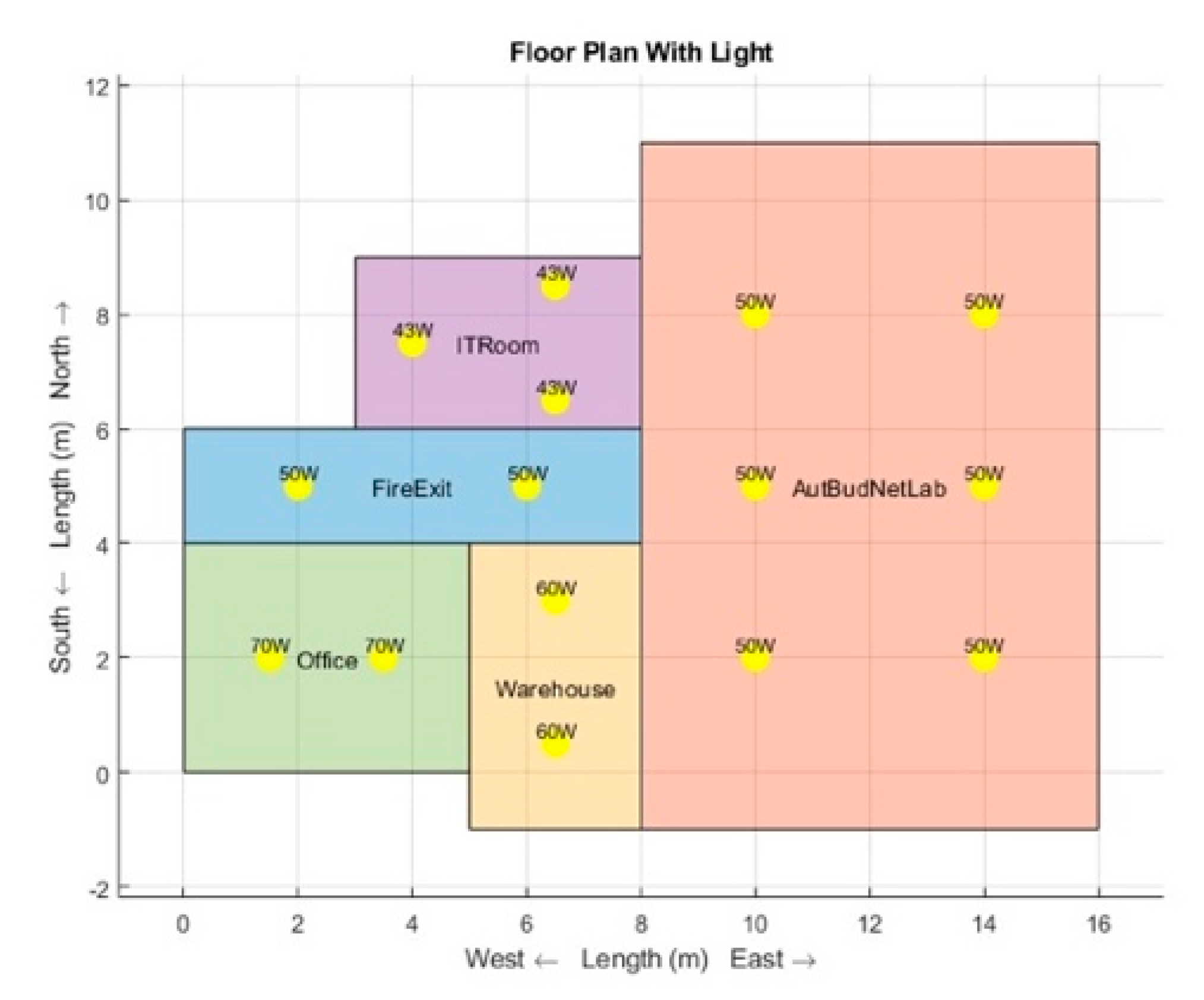
Figure 2.
3D model of the simulated building.
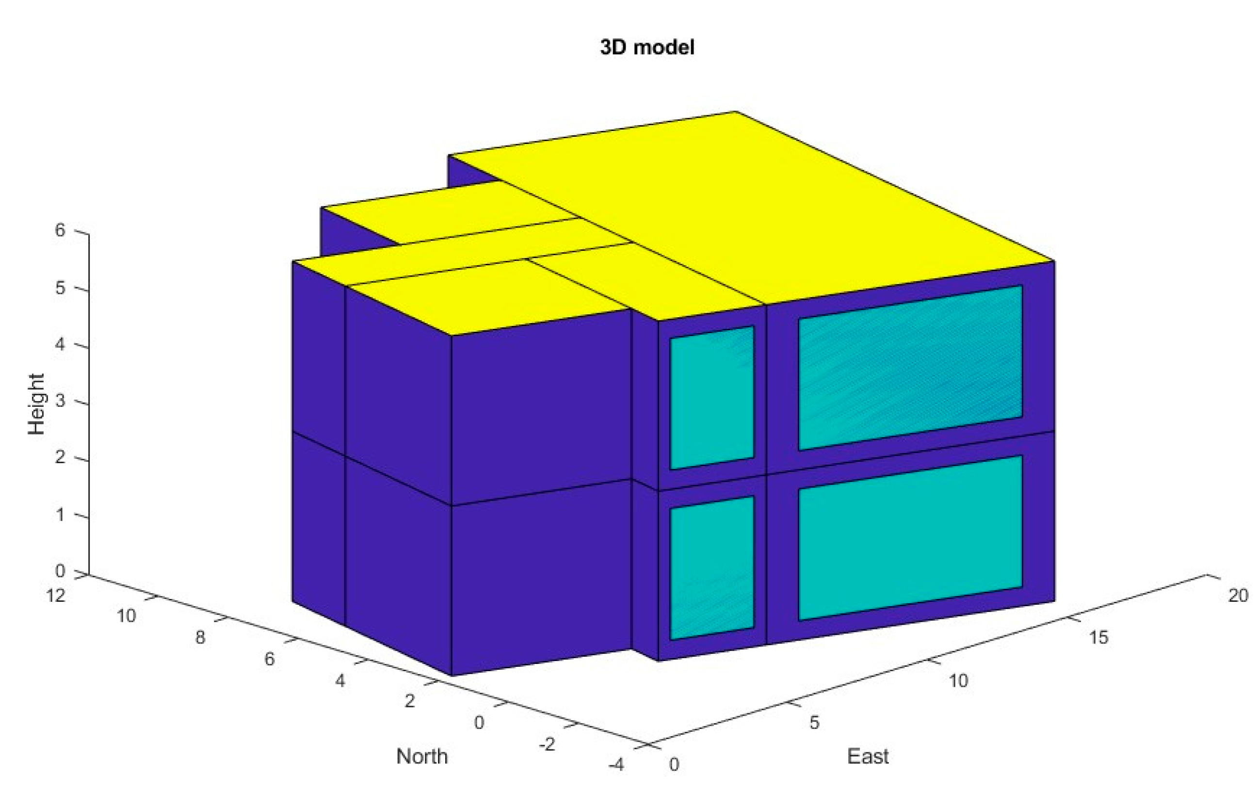
Figure 3.
The occupancy patterns in the rooms on all floors.
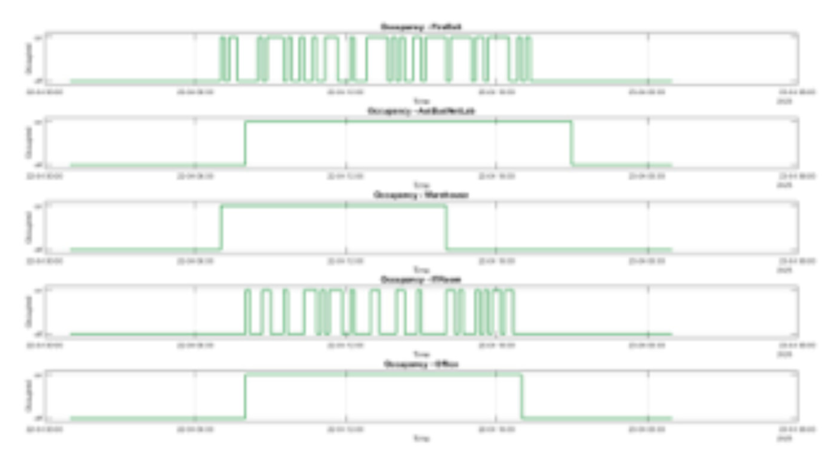
Figure 4.
Total occupancy hours.
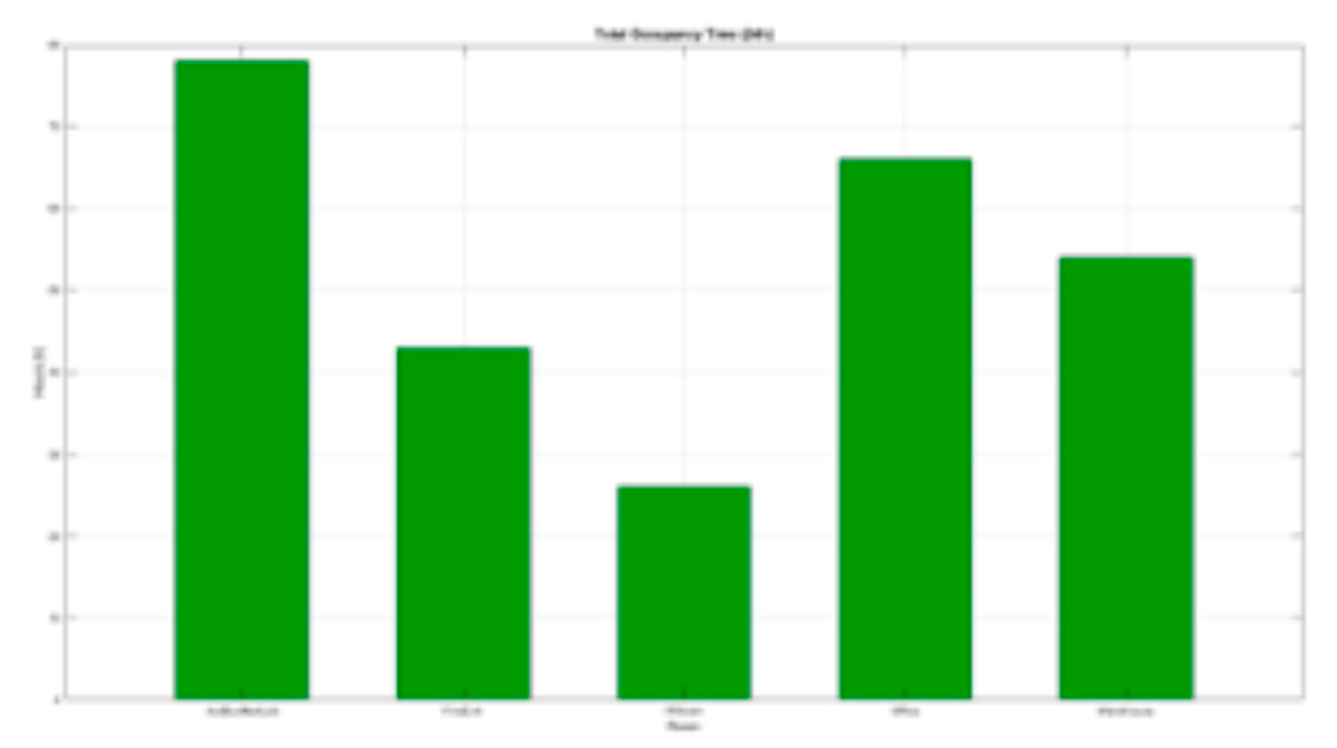
Figure 5.
HVAC system model: (a) General diagram of the model; (b) Block diagram of the digital twin control system.
Figure 5.
HVAC system model: (a) General diagram of the model; (b) Block diagram of the digital twin control system.
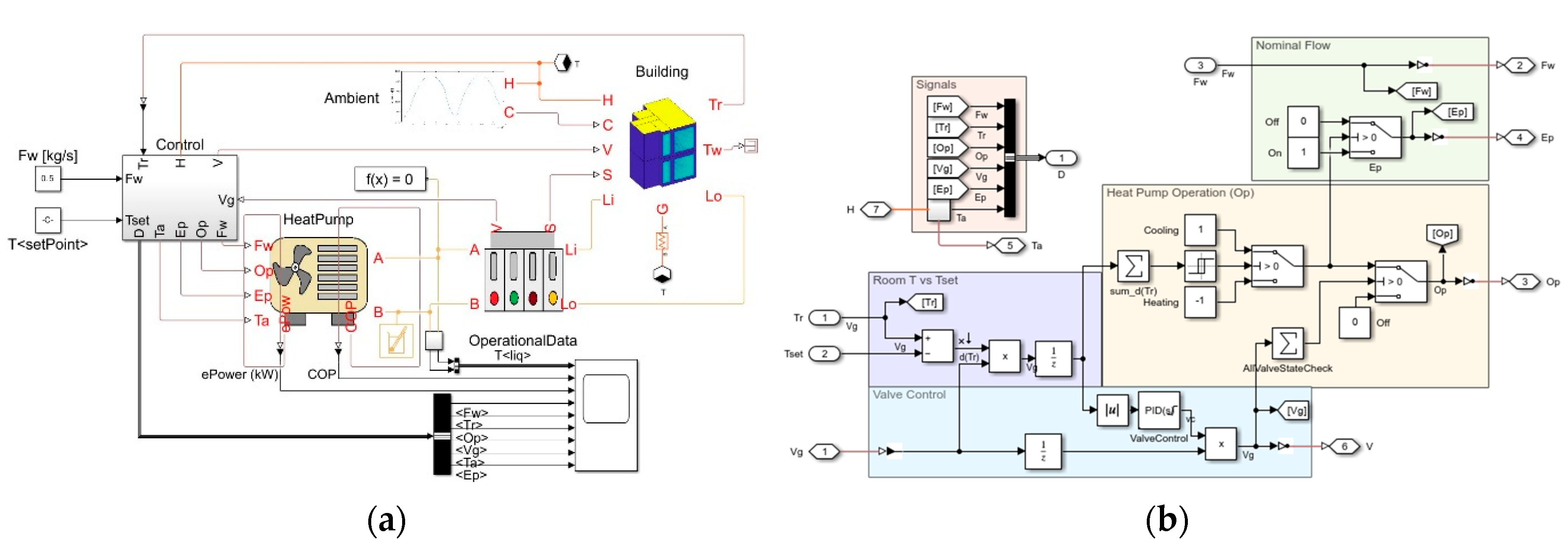
Figure 6.
24 hour HVAC energy consumption profiles with cumulative energy use level for Scenario A (Class C).
Figure 6.
24 hour HVAC energy consumption profiles with cumulative energy use level for Scenario A (Class C).
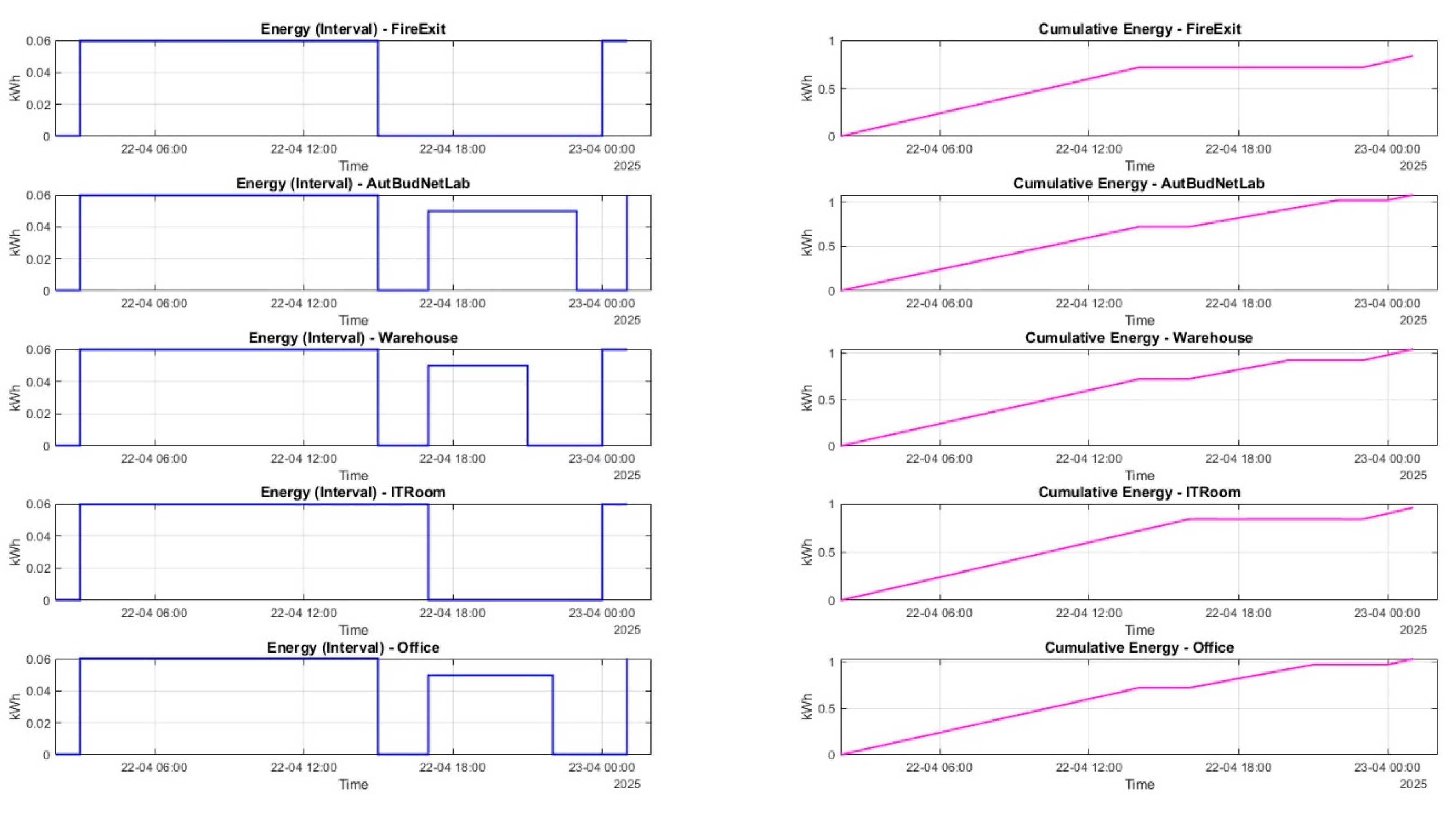
Figure 7.
HVAC power and temperature trajectories for Scenario A (Class C). Time-series plot illustrating heating power pulses required to maintain the fixed 17 °C setpoint, absence of cooling activation, and stable zone temperatures.
Figure 7.
HVAC power and temperature trajectories for Scenario A (Class C). Time-series plot illustrating heating power pulses required to maintain the fixed 17 °C setpoint, absence of cooling activation, and stable zone temperatures.
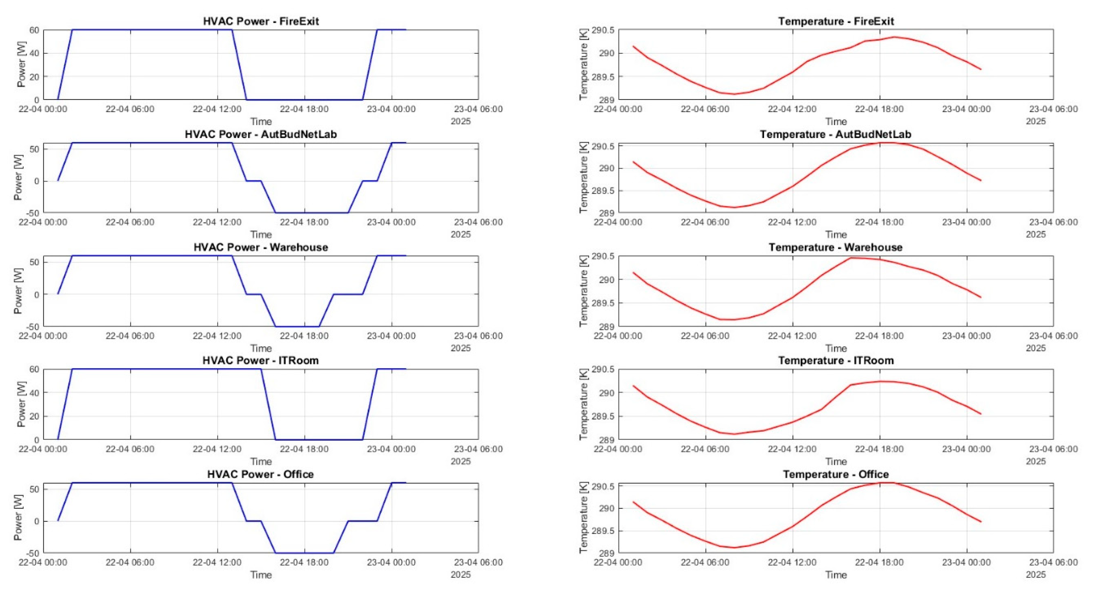
Figure 8.
Lighting operation profiles for rooms in Scenario A (Class C). Time-series plot showing binary on/off activation of luminaires in all occupied zones throughout the 24-hour simulation period.
Figure 8.
Lighting operation profiles for rooms in Scenario A (Class C). Time-series plot showing binary on/off activation of luminaires in all occupied zones throughout the 24-hour simulation period.
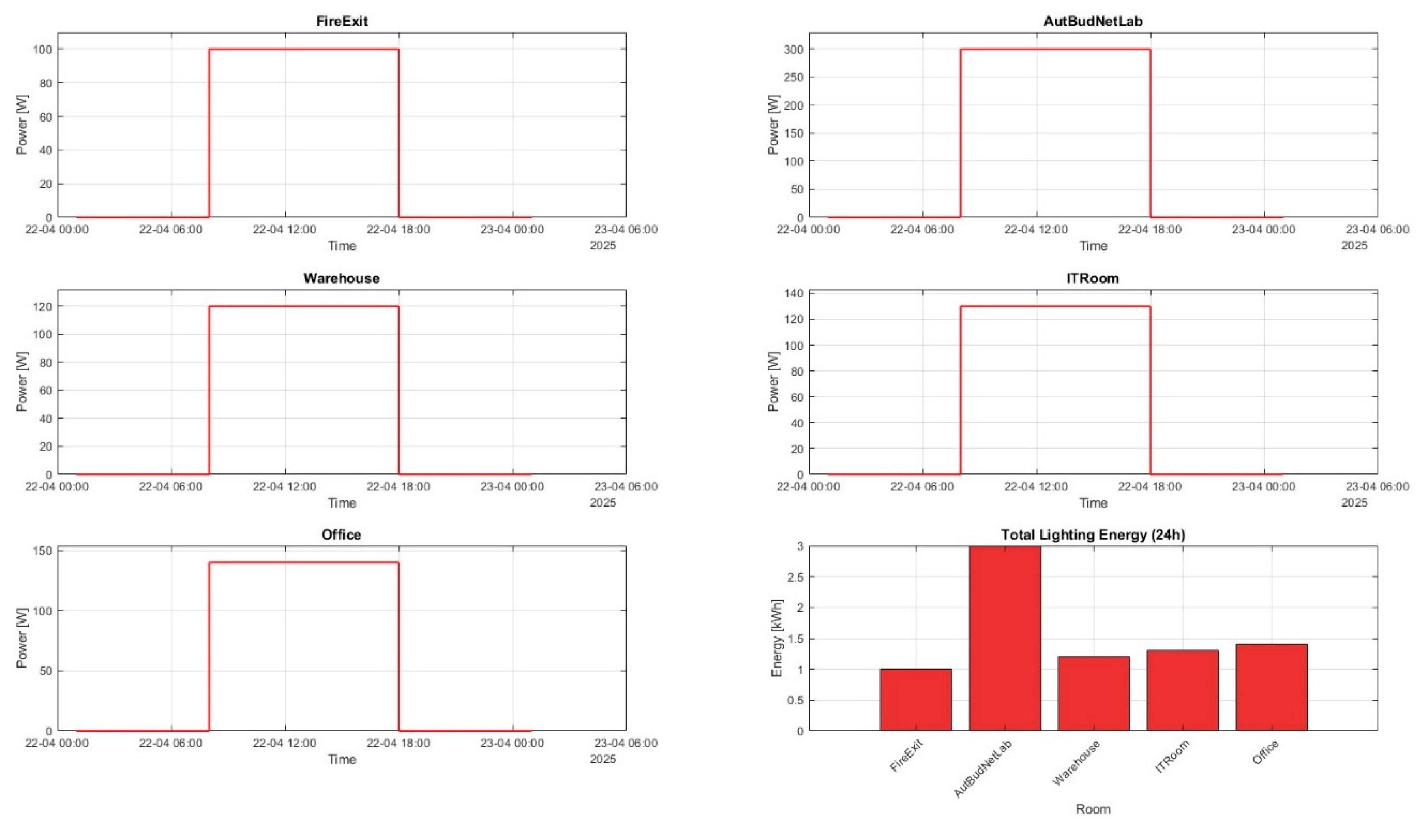
Figure 9.
24-hour HVAC energy consumption profiles with cumulative energy use level for Scenario B (Class A).
Figure 9.
24-hour HVAC energy consumption profiles with cumulative energy use level for Scenario B (Class A).
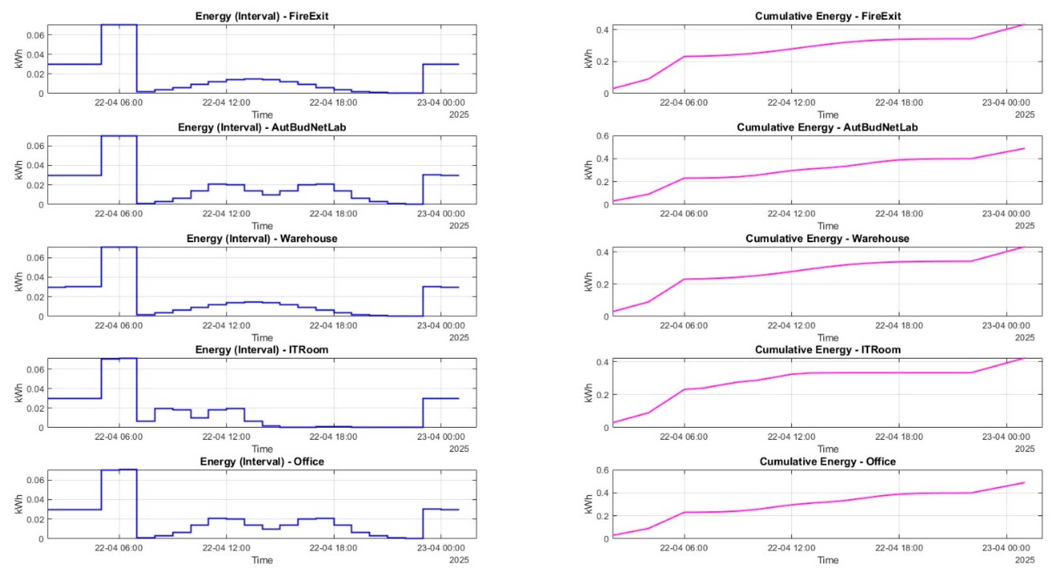
Figure 10.
HVAC power and temperature trajectories for Scenario B (Class A).
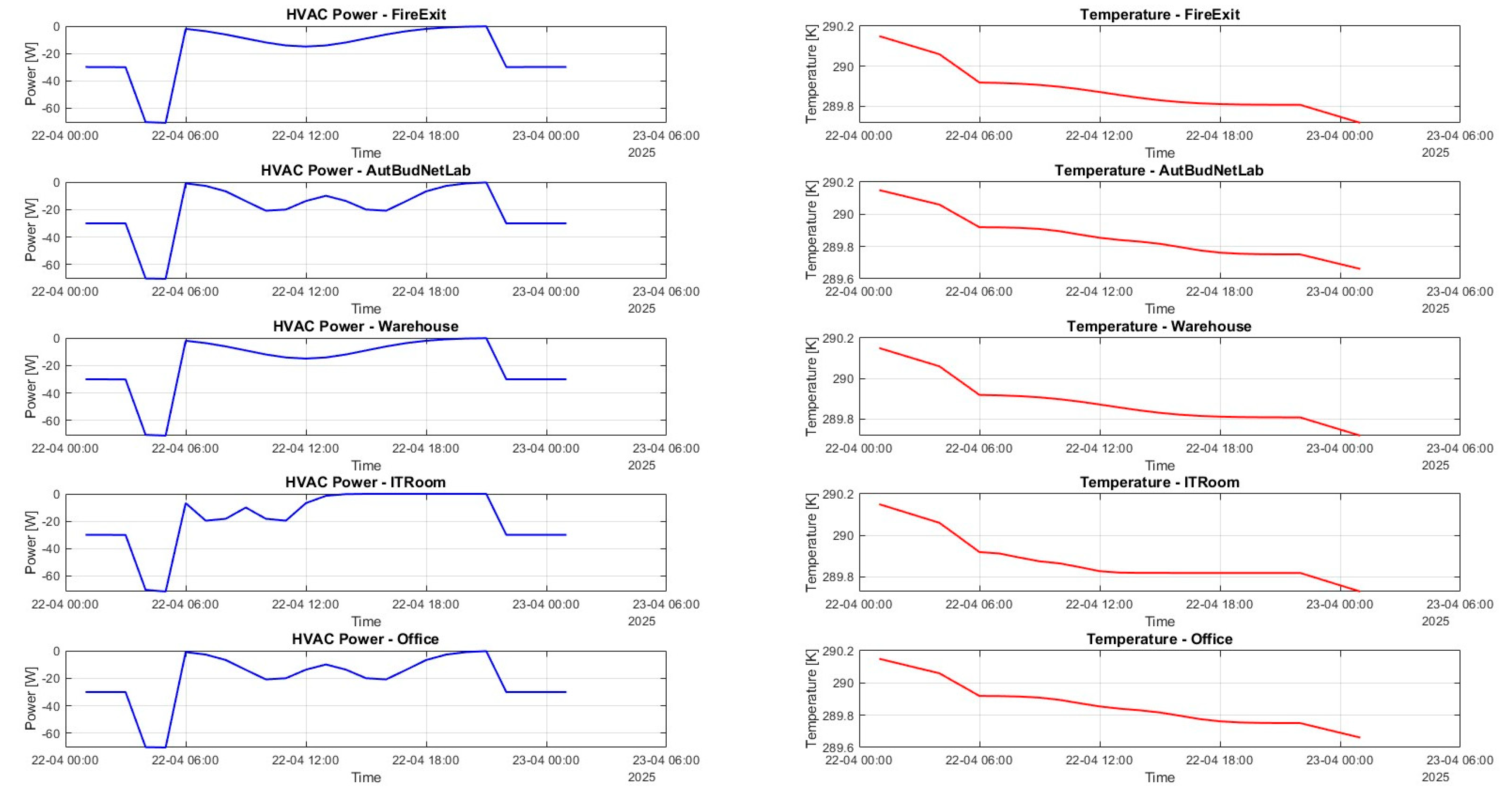
Figure 11.
Lighting operation profile for Scenario B (Class A). Time-series plot showing binary on/off activation of luminaires in all occupied zones across the 24-hour simulation period.
Figure 11.
Lighting operation profile for Scenario B (Class A). Time-series plot showing binary on/off activation of luminaires in all occupied zones across the 24-hour simulation period.
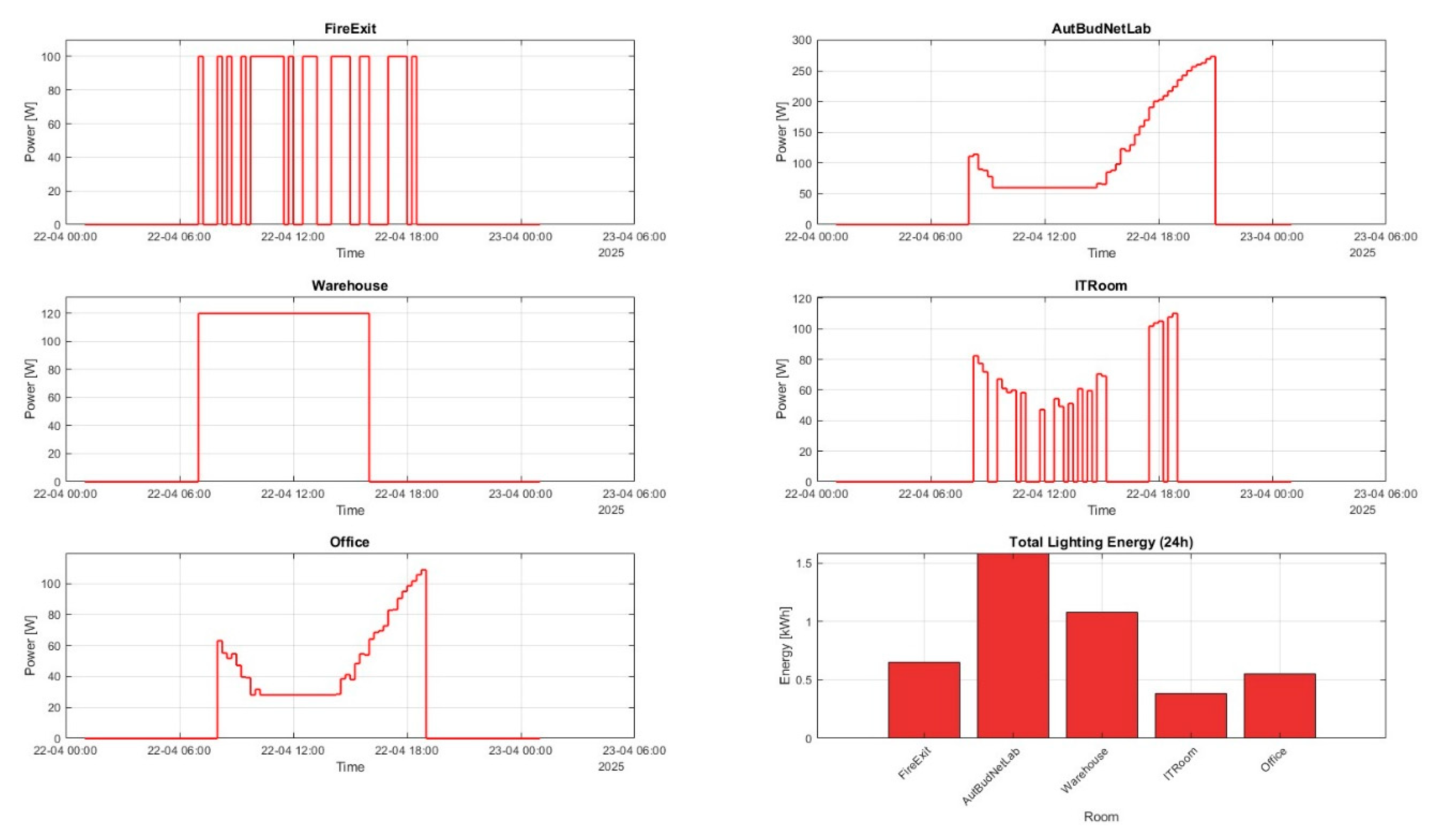
Figure 12.
24-hour HVAC energy consumption profiles with cumulative energy use level for Scenario C (high SRI level).
Figure 12.
24-hour HVAC energy consumption profiles with cumulative energy use level for Scenario C (high SRI level).
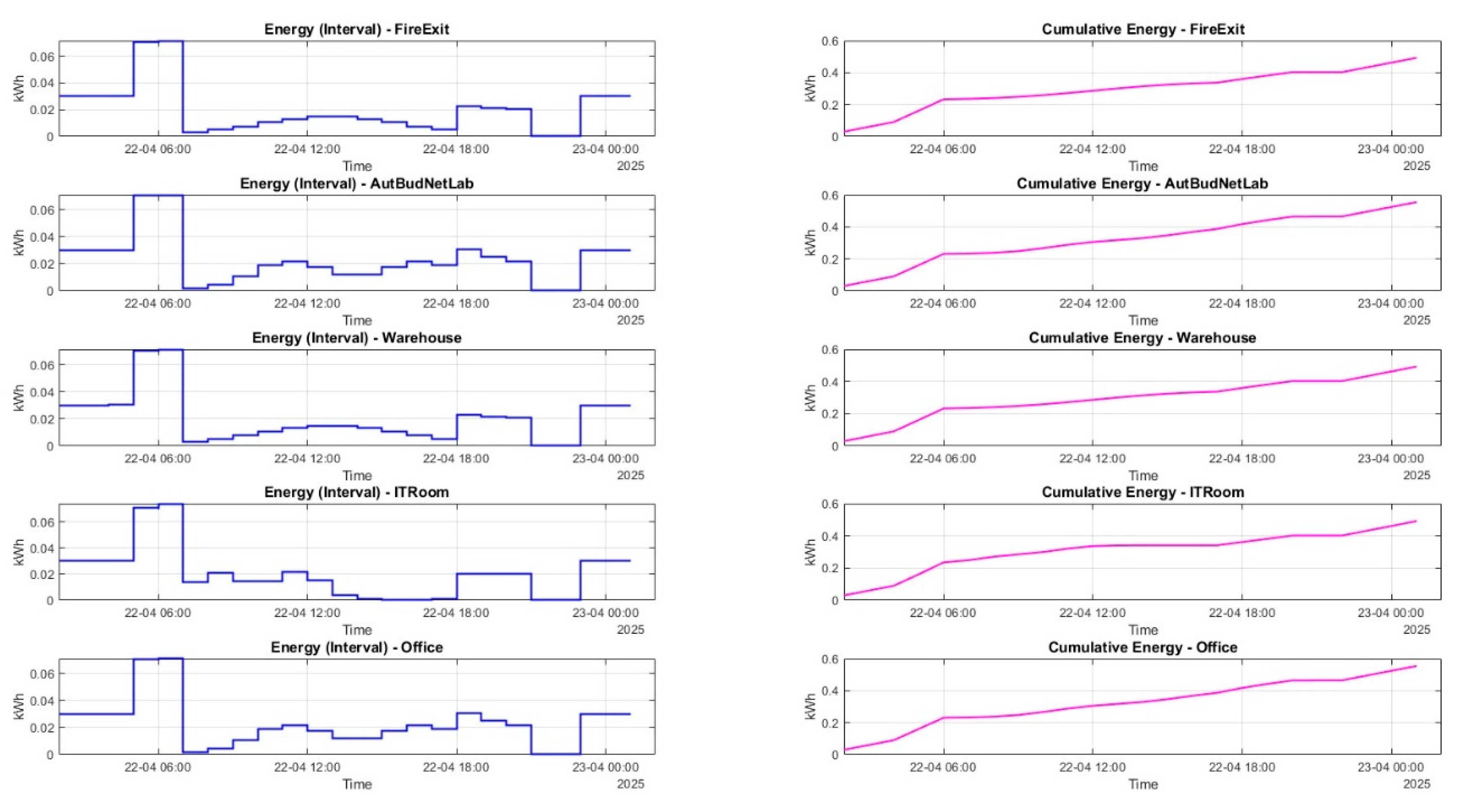
Figure 13.
HVAC power and temperature trajectories for Scenario C (high SRI level): (a) Scenario C with active blind control; (b) Scenario C without blinds control.
Figure 13.
HVAC power and temperature trajectories for Scenario C (high SRI level): (a) Scenario C with active blind control; (b) Scenario C without blinds control.
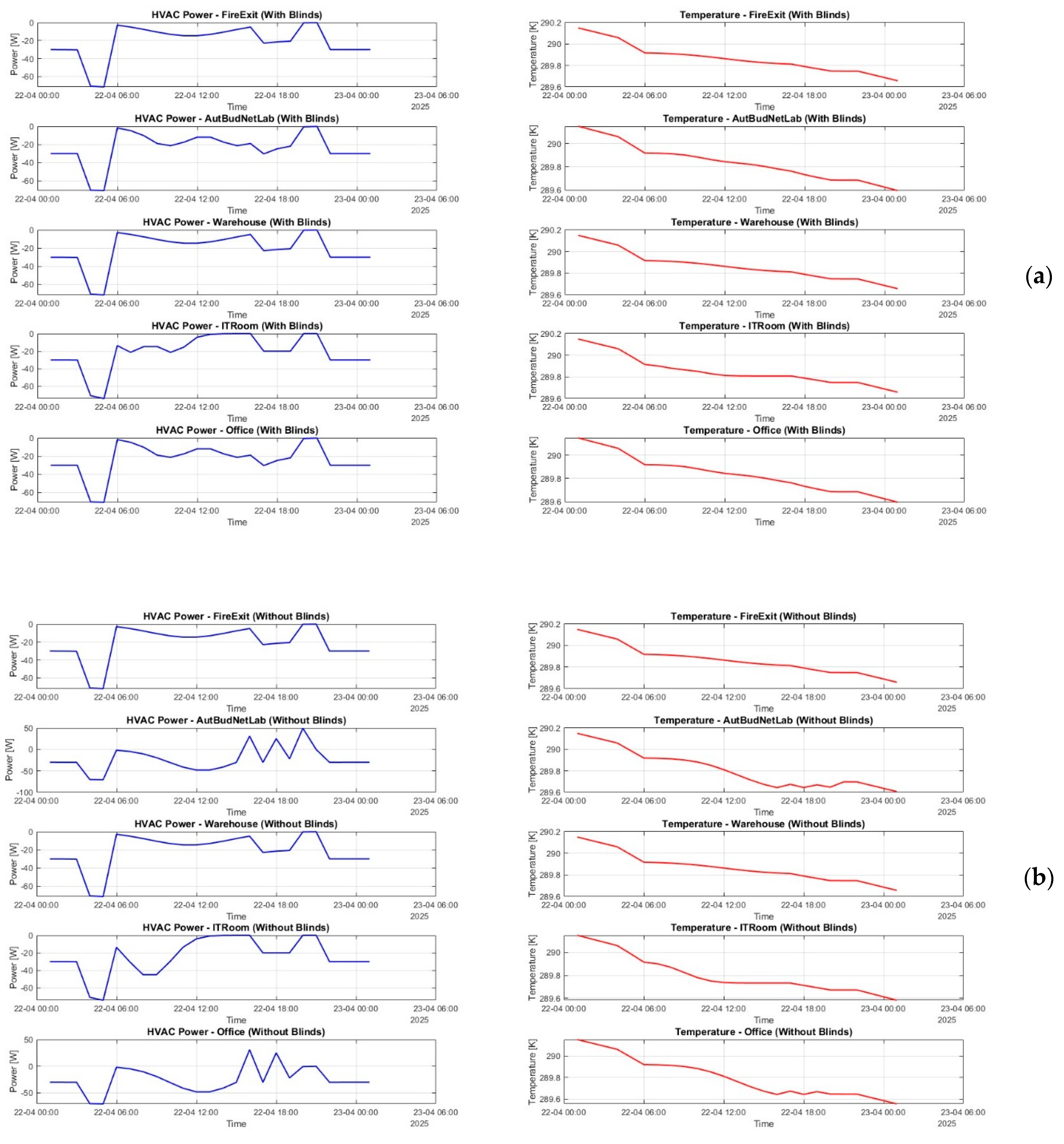
Figure 14.
Lighting operation profile for Scenario C (high SRI level). Time-series plot showing binary on/off activation of luminaires in all occupied zones across the 24-hour simulation period.
Figure 14.
Lighting operation profile for Scenario C (high SRI level). Time-series plot showing binary on/off activation of luminaires in all occupied zones across the 24-hour simulation period.
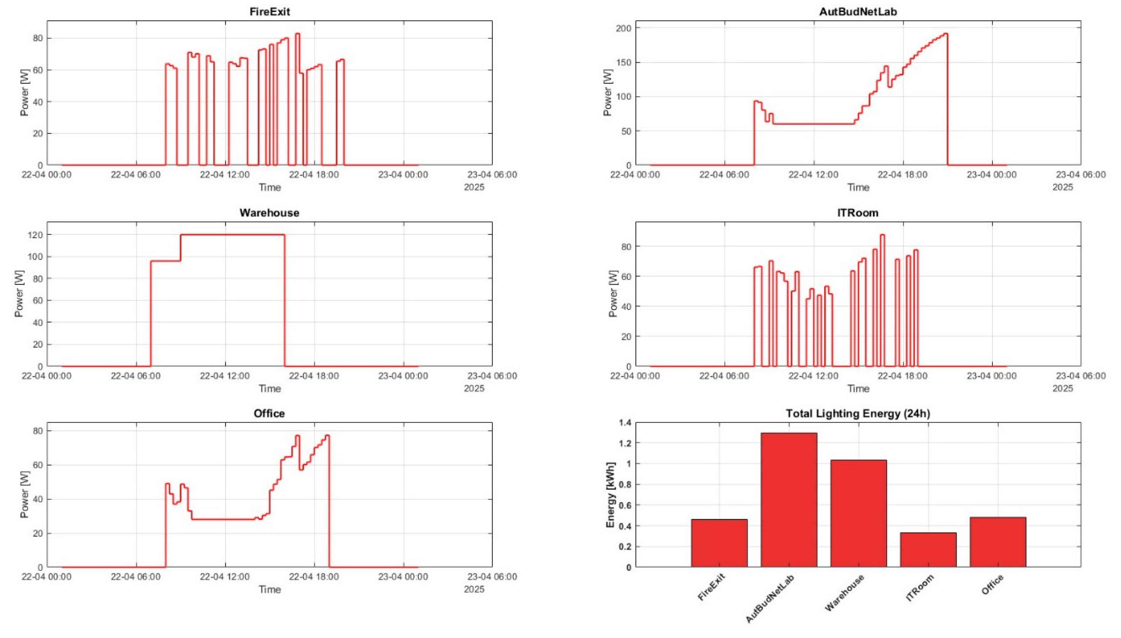
Figure 15.
Comparison of total energy use and subsystem energy distribution (HVAC and lighting) across the three automation scenarios: (a) Energy use – general comparison; (b) Energy use by systems – comparison.
Figure 15.
Comparison of total energy use and subsystem energy distribution (HVAC and lighting) across the three automation scenarios: (a) Energy use – general comparison; (b) Energy use by systems – comparison.
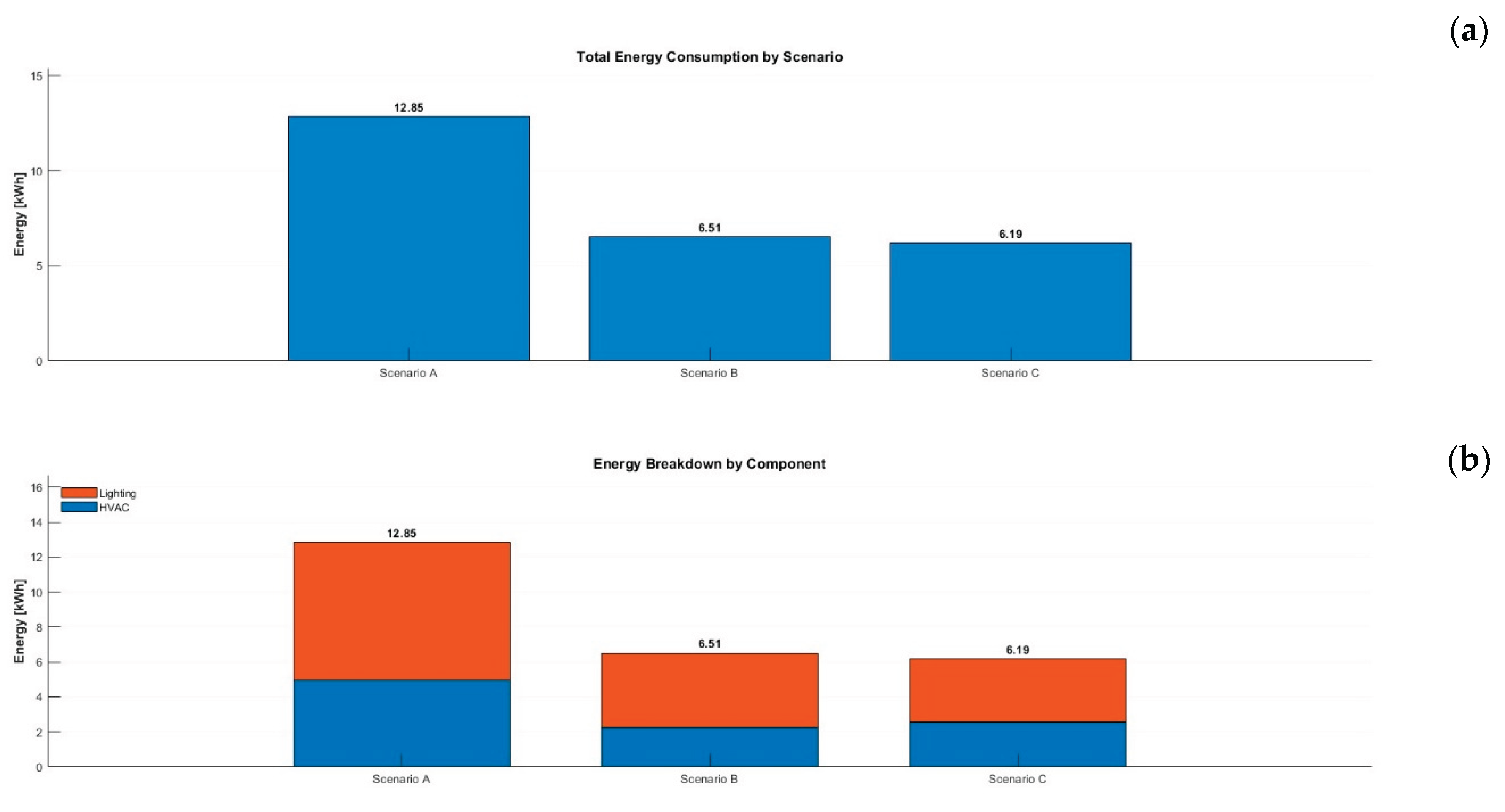
Figure 16.
Comparative analysis of energy consumption, illustrating 24-hour versus weekly energy utilization profiles with detailed breakdown of HVAC and lighting system contributions.
Figure 16.
Comparative analysis of energy consumption, illustrating 24-hour versus weekly energy utilization profiles with detailed breakdown of HVAC and lighting system contributions.
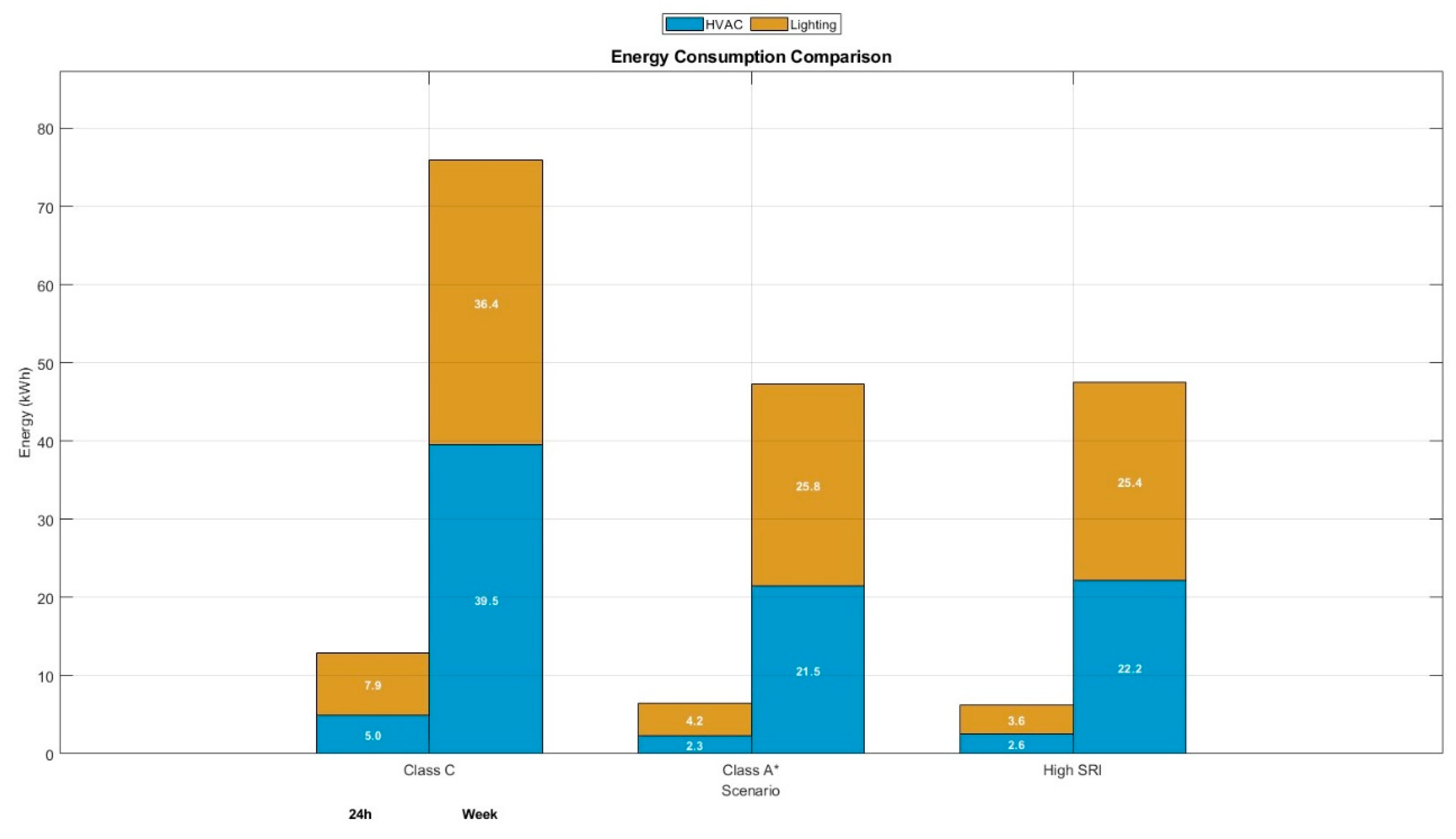

Table 1.
Comparative overview of selected DT and BACS studies relevant to the evaluation of smart building with different simulation approaches.
Table 1.
Comparative overview of selected DT and BACS studies relevant to the evaluation of smart building with different simulation approaches.
| Study/Case | DT-BIM Integration | Standard/Framework Alignment |
Simulation Environment |
Quantitative Assessment (e.g., EN ISO 52120 or SRI Method C) |
| DanRETwin [2] | Full BIM–DT coupling, real sensor data | Partial EN ISO 52120 mapping |
MATLAB / Simulink + AI modules |
Energy & comfort validation based on measured vs simulated data |
| Comfort-DT Framework [9] | BIM-based thermal and control models |
Focus on DT/BIM comfort optimization, without formal standard reference | MATLAB / Simulink |
Scenario-based evaluation of HVAC & lighting automation |
| Smart District Readiness Pilot [18] | Multi-buildings modeling (district aggregation) |
Full EN ISO 52120 + SRI integration |
TRNSYS + custom Python scripts |
Load-shifting and SRI-score quantification |
| Hybrid BACS Model [25] | Simplified BIM inputs, parametric control layers | EN ISO 52120 aligned with SRI analysis |
MATLAB / Simulink |
BACS Function-level energy impact and SRI-related performance |
| SRI Review Framework [12] | Conceptual DT representation |
SRI Method C discussion | Mixed methods (survey + simulation) |
Proposal of a quantitative smart-readiness evaluation pathway |
Table 2.
Total lighting power per room.
| Room | Total Power [W] |
| AutBudNet Lab | 300 |
| Fire Exit | 100 |
| IT Room | 129 |
| Office | 140 |
| Warehouse | 120 |
Table 3.
System control strategy in Scenario A (Class C from EN ISO 52120).
| System | Control strategy |
| Heating | Setpoint constant 17 °C; individual room control |
| Cooling | The activation threshold is set at the set point in the room of 17 °C. Due to the low setpoint and the Polish climate conditions, cooling activation is highly improbable. |
| Ventilation and AC | On/off based on occupancy; fixed airflow; no demand control |
| Lighting | On/off via occupancy detection and manual switch; no daylight harvesting and dimming control |
| Solar gain (blinds) | Manual motorized control; no automatic shading |
| Energy reporting | Basic HVAC runtime logs; no grid interaction; the building operates independently from grid signals |
Table 4.
Energy consumption in Scenario A.
| System | Energy [kWh] | Share |
| HVAC | 4.95 | 38.5% |
| Lighting | 7.90 | 61.5% |
| Total | 12.85 | 100% |
Table 5.
Room-specific energy consumption in Scenario A.
| Room | HVAC [kWh] | Lighting [kWh] | Total [kWh] |
| AutBudNet Lab | 1.08 | 3.00 | 4.08 |
| FireExit | 0.84 | 1.00 | 1.84 |
| IT Room | 0.96 | 1.30 | 2.26 |
| Office | 1.03 | 1.40 | 2.43 |
| Warehouse | 1.04 | 1.20 | 2.24 |
Table 6.
System control strategy in Scenario B (Class A from EN ISO 52120).
| System | Control strategy |
| Heating | Adaptive deadband (0.5 °C), heat recovery from exhaust air, occupancy-linked adjustments with and inter-room communication |
| Cooling | Free cooling through night ventilation (when the outdoor temperature is below 17 °C) and pre-cooling at dawn to reduce peak daytime cooling loads |
| Ventilation and AC | Occupancy-proportional airflow (Demand-Controlled Ventilation), humidity-triggered boost to prevent condensation (e.g., at 9 °C nights) |
| Lighting | Daylight-aware dimming – artificial light intensity is modulated based on available natural light, with sensitivity adjusted for orientation (e.g., south zones brighter), automatic detection for turn-off, but requires manual on |
| Solar gain (blinds) | Automatic dimming of the solar gain based on insolation, the system combined light/blind/HVAC control – ventilation offsets potential overheating (e.g., via extra airflow in south-facing zones).” |
| Energy reporting | Advanced zone-by-zone monitoring with temperature deviation alerts and centralized fault detection/diagnostics, active Demand-Side Management (DSM) for load shifting based on grid load signals |
Table 7.
Energy consumption in Scenario B.
| Scenario Variant | HVAC [kWh] | Lighting [kWh] | Total [kWh] |
| Scenario B (With Blinds) | 2.27 | 4.25 | 6.52 |
| Scenario B (No Blinds) | 2.24 | 4.25 | 6.49 |
| Difference (Δ) | +0.03 | 0.00 | +0.03 |
Table 8.
Room-specific energy consumption in Scenario B with blind control.
| Room | HVAC [kWh] | Lighting [kWh] | Total [kWh] |
| AutBudNet Lab | 0.49 | 1.60 | 2.09 |
| FireExit | 0.43 | 0.65 | 1.08 |
| IT Room | 0.42 | 0.35 | 0.77 |
| Office | 0.50 | 0.55 | 1.05 |
| Warehouse | 0.43 | 1.10 | 1.53 |
Table 9.
System control strategy in Scenario C (High SRI Level).
| System | Control strategy |
| Heating | Individual room control with presence detection, features centralized monitoring with forecasting, benchmarking, predictive management, and fault detection |
| Cooling | Occupancy-aware zone control with demand-driven pumps and dynamic grid-responsive sequencing, cooling optimized via MPC, integrating performance evaluation, forecasting, and fault detection |
| Ventilation and AC | Local demand control utilizing air quality sensors (CO2, VOC – Volatile Organic Compound), with precise airflow modulation via dampers |
| Lighting | Automatic dimming with time-based, adaptive lighting scenes that dynamically adjust illuminance, color, and light distribution to specific design requirements, tasks, and user needs |
| Solar gain (blinds) | Predictive blind control based on external data sources, such as weather forecasts, to manage solar gain proactively before conditions change |
| Energy reporting | Comprehensive performance evaluation incorporating forecasting, benchmarking, predictive management, and integrated fault detection |
Table 10.
Energy consumption in Scenario C.
| Scenario Variant | HVAC [kWh] | Lighting [kWh] | Total [kWh] |
| Scenario B (With Blinds) | 2.59 | 3.60 | 6.19 |
| Scenario B (No Blinds) | 3.01 | 3.60 | 6.61 |
| Difference (Δ) | +0.42 | 0.00 | +0.42 |
Table 11.
Room-specific energy consumption in Scenario C with blinds control.
| Room | HVAC [kWh] | Lighting [kWh] | Total [kWh] |
| AutBudNet Lab | 0.56 | 1.30 | 1.85 |
| FireExit | 0.49 | 0.46 | 0.95 |
| IT Room | 0.49 | 0.33 | 0.83 |
| Office | 0.56 | 0.48 | 1.03 |
| Warehouse | 0.49 | 1.03 | 1.52 |
Table 12.
Weekly energy consumption.
| Scenario | HVAC [kWh] | Lighting [kWh] | Total [kWh] |
Savings vs. Scenario A |
| A – Class C EN ISO 52120 |
39.54 | 36.38 | 75.92 | - |
| B – Class A EN ISO 52120 |
21.53 | 25.78 | 47.31 | 28.61 [kWh] (37.7%) |
| C – High SRI level | 22.19 | 25.36 | 47.55 | 28.37 [kWh] (37.4%) |
Disclaimer/Publisher’s Note: The statements, opinions and data contained in all publications are solely those of the individual author(s) and contributor(s) and not of MDPI and/or the editor(s). MDPI and/or the editor(s) disclaim responsibility for any injury to people or property resulting from any ideas, methods, instructions or products referred to in the content. |
© 2025 by the authors. Licensee MDPI, Basel, Switzerland. This article is an open access article distributed under the terms and conditions of the Creative Commons Attribution (CC BY) license (http://creativecommons.org/licenses/by/4.0/).
Copyright: This open access article is published under a Creative Commons CC BY 4.0 license, which permit the free download, distribution, and reuse, provided that the author and preprint are cited in any reuse.


