
Submitted:
08 December 2025
Posted:
09 December 2025
You are already at the latest version
Abstract
The critical micelle concentration (CMC) is a fundamental physicochemical property of surfactants with significant implications across multiple industries. This paper presents uncertainty-aware graph neural network that integrates molecular structure and temperature to simultaneously predict CMC values and prediction uncertainties. Trained on a curated dataset of 1,829 surfactants with temperature annotations, our GNN achieves competitive performance (RMSE = 0.352, MAE = 0.244) on an external test set, outperforming previous models in RMSE. The model provides statistically sound, adequately calibrated uncertainty estimates that reliably quantify prediction confidence. This dual-output approach enables reliable CMC prediction with quantifiable confidence intervals, addressing a practical need for safety-critical applications where underestimation of uncertainty could have serious consequences.
Keywords:
surfactants
; critical micelle concentration
; CMC
; CMC prediction
; machine learning
; ML
; graph neural network
; GNN
; model uncertainty
1. Introduction
The critical micelle concentration (CMC) is one of the most important physicochemical properties of surfactants, with significant implications in the cosmetic, pharmaceutical, household, mining and gas&oil industries. The CMC is directly or indirectly related to surfactant’s surface activity, effective concentration, toxicity, biological activity, and other key characteristics. Due to the considerable structural diversity of surfactants, no comprehensive theoretical methods currently exist to predict CMC as a function of molecular structure.
Molecular dynamics (MD) and quantum-chemical based quantitative structure-property relationship (QSPR) models have been previously employed for CMC prediction. Turchi et al. [1] presented a newly developed method, which employs first principles-based interfacial tension calculations rooted in quantum chemical COSMO-RS theory, for the prediction of the critical micelle concentration of a set of nonionic, cationic, anionic, and zwitterionic surfactants in aqueous solutions. Cárdenas et al. [2] determined interfacial tension and CMC of sugar-based nonionic surfactant n-dodecyl glucoside from atomistic molecular simulations; approximated value of the CMC was obtained by geometrical analysis of the behavior of the interface.
Additionally, group-contribution methods and probabilistic approaches, including Markov chain modeling, have been applied for surfactant’s CMC prediction. Mattei et al. [3] developed an extended group-contribution model for predicting CMC values of nonionic surfactants in aqueous solutions at 25 °C. Smith et al. [4] employed a Markov chain model to predict CMC and surface composition in binary surfactant systems.
Conventional QSPR methods – relying on quantum chemical calculations, molecular dynamics simulations or other non-machine learning (non-ML) techniques – often entail high computational costs and remain limited in their ability to incorporate the influence of structural features. In contrast, cheminformatics has emerged as a robust paradigm for molecular design and property prediction, leveraging data-driven models to analyze chemical data of varying scales and complexity.
Machine learning (ML) has become an established tool in cheminformatics, demonstrating success in solving various problems [5,6,7,8], including CMC prediction. Early attempts at utilizing ML models for CMC prediction mostly are multiple linear regression (MLR) models used with different types of descriptors – topological [9,10], quantum-chemical [11,12] or their combination [13] for CMC prediction of single type surfactants (mostly nonionic or anionic). Subsequent research expanded descriptor diversity to include fragment-based and structural features [14,15]. A notable exception among them is the partial least squares (PLS) regression model by Anoune et al. [16], which was trained on a combination of different types of descriptors – ranging from compound molecular weight to various electrical (e.g., dipole moment) and topology-dependent properties – to predict CMC of multiple surfactant types. The methodological advancement continued with the adoption of artificial neural networks (ANN) [17,18,19,20], support vector regression (SVR) [15,18,20] and tree-based [20] methods, each demonstrating enhanced predictive capability for structurally diverse surfactants.
Latest advances in the field have focused on graph neural networks (GNNs) [21,22,23], which directly process molecular graph representations to capture complex structural relationships without predefined descriptors, thereby improving generalizability across diverse surfactant structures. The GNN model by Moriarty et al. [22] was augmented with Gaussian processes (GNN/GP) to implement an uncertainty quantification technique that yields confidence intervals alongside CMC predictions. In this case, GNN is trained to produce a latent representation vector for each molecule and then gaussian processes is trained on these standardized latent representations to predict normal distribution for the CMC value, where μ is the predicted mean CMC value and σ is the predicted standard deviation, representing the uncertainty.
While molecular structure fundamentally determines surfactant behavior, CMC property exhibits significant dependence on environmental parameters, most notably temperature. Temperature-dependent modeling has been performed by various researchers by implementing GNNs [24,25], tree-based ensemble methods [26] and ANN with quantum-chemical descriptors [27]. Among these, single property prediction Attentive FP model by Hodl et al. [25] was able to achieve state-of-the-art CMC prediction performance with mean absolute error (MAE) of 0.241 and root mean squared error (RMSE) of 0.365. Their multiproperty models, predicting pCMC, the surface tension at the CMC (γCMC), surface excess concentration (Гmax × 106) and the surfactant efficiency (pC20), achieved even better CMC prediction results of MAE = 0.235, RMSE = 0.346.
To the best of our knowledge, none of Hodl et al. models’ have the ability to predict uncertainty alongside the actual prediction, and the only implementation predicting both CMC and model uncertainty is reported in Moriarty et al. temperature-independent GNN/GP model [22].
Methodological advancements in CMC prediction were accompanied by the problems of data scarcity. Early datasets were limited to approximately 200 experimentally determined values, predominantly comprising nonionic surfactants with limited structural diversity [13]. While presently reported datasets have expanded to encompass more than 1,000 data points spanning multiple surfactant classes [24,25,27], the field continues to face challenges related to data diversification, inconsistent experimental conditions, and underrepresentation of certain surfactant categories.
This work aims to address the problem of data scarcity by incorporating and processing datasets from multiple open sources. The processed dataset is utilized for training descriptor-based models and previously reported GNN models, initially trained for reaction atom-to-atom mapping [28] and used to solve problems in other fields [29,30,31], but previously not applied to CMC determination. Descriptor-based models are trained and tested to establish a baseline for GNN models. During the training process, the developed GNN model learns to not only accurately predict surfactant's CMC at a given measurement temperature, but to also adequately assess its own uncertainty. The predictive ability of the trained models was tested using the SurfPro test set and compare our findings with the results reported on the same test set by Hodl et al. [25].
2. Materials and Methods
2.1. Fingerprint-Based Machine Learning Models
To assess the quality of the processed dataset, fingerprint-based machine learning models were trained and evaluated. Molecular fingerprints of 4096 bits were generated using the RDKit [32] Fingerprint (FP) generator, with a path length range of 2 to 12 bonds.
The selection of path length range of 2 to 12 bonds, and FP size of 4096 bits for molecular FP generation was driven by empirical analysis of feature distribution in the processed dataset. Assessment metrics revealed the following trade-offs: shorter path lengths (e.g., max path of 6) yielded excessive rare features (1,543 bits present in < 10% of molecules), indicating insufficient structural resolution for diverse surfactants. Conversely, longer paths (max path of 16) generated overwhelming redundancy (554 bits in > 50% of molecules), obscuring discriminative chemical motifs. The max path of 12 optimally balanced these extremes, capturing characteristic surfactant substructures while avoiding over-representation. Doubling FP size from 2048 to 4096 at max path of 12 further refined this balance, reducing overrepresented bits from 193 to 107, indicating enhanced feature discriminability without excessive sparsity.
Generated molecular fingerprints served as input features for two regression models: Random Forest Regressor (RF) and XGBoost Regressor (XGB). Input features did not include CMC measurement temperature. For training and testing of most of the models “scikit-learn” version 1.7.1 [33] was used, for XGBoost models “xgboost” version 3.0.5 [34] was used. Molecular FPs were generated using “rdkit” version 2025.3.5 [32].
2.2. Graph Neural Network
The described model implements a hierarchical deep learning architecture for predicting CMC from molecular structures. Our GNN’s architecture is designed to model both the target property and its predictive uncertainty [35] simultaneously. Canonical SMILES of surfactants get converted to molecular graphs via Chython library, version 1.78 [36], which are then passed on to Chytorch, version 1.57 [37] MoleculeEncoder based on Graphormer principles from the rxnmap [38] pretrained model (version 1.4) of Chytorch zoo module [28].
MoleculeEncoder processes molecular graphs through atom, neighbor, and distance embeddings to generate a comprehensive 1024-dimensional representation. This representation captures complex structural and topological features through multi-head attention mechanisms within the Graphormer layer, enabling the model to discern relevant molecular patterns critical for CMC prediction. The general molecular representation is extracted via Slicer operation (from Chytorch) and subsequently refined through a five-layer MLP (1024→512→256→128→64→32) with ReLU/PReLU activations and progressive dropout regularization (rates decreasing from 0.3 to 0.2). This encoder pathway effectively distills the high-dimensional graph representation into a compact, information-rich molecular fingerprint optimized for property prediction.
Concurrently, the temperature input (a scalar value) is processed by a separate Multilayer perceptron (MLP) that maps it to a m-dimensional feature vector. This network consists of 3 linear layers with batch normalization and PReLU activations, designed to capture non-linear relationships between temperature and log CMC mol/L. The exploration of multiple temperature MLP architectures (1→2→4, 1→8→8, 1→8→16) was systematically undertaken to identify an optimal balance between model complexity and the inherent information capacity of the single-dimensional temperature variable. This experimental design was grounded in several considerations: first, to evaluate how different embedding dimensions affect the model's ability to represent the non-linear temperature dependence of CMC; second, to ensure dimensional compatibility with the molecular 32 feature space while preventing over-parameterization; and third, to identify the minimal embedding dimension that maintains sufficient representational capacity without introducing unnecessary complexity. The specific architectures chosen represent a geometric progression of increasing complexity, allowing for systematic analysis of capacity-accuracy trade-offs while maintaining computational efficiency.
The molecular and temperature features are concatenated and fed into a final MLP that produces a two-dimensional output: the predicted log CMC value and a log-variance term. The log-variance is used to model heteroscedastic uncertainty, allowing the model to predict a confidence interval for each prediction. The GNN architecture is schematically presented on Figure 1.
Unlike uncertainty implementation in Moriarty et al. GNN/GP model [22], which represents a two-stage approach, our model implements an end-to-end approach where the model is trained to directly predict both CMC and uncertainty. Moriarty's approach excels at providing theoretically sound uncertainty estimates that reflect the model's confidence based on proximity to training data in chemical space. Our GNN model implementation described above prioritizes practical implementation and computational efficiency, directly predicting uncertainty as part of the model's output.
This GNN model implementation represents a strategic application of transfer learning methodology, which is particularly advantageous given the limited availability of experimentally determined CMC reference data. The rxnmap model, originally trained on USPTO and Pistachio reaction datasets and described in detail by Nugmanov et al. [28], possesses extensive prior knowledge of chemical space topology through its bidirectional graph transformer architecture. Rather than learning chemical representation de novo, the transfer learning approach effectively constrains the optimization problem to identifying the hyperplane that optimally describes log CMC property relationships within the pre-established chemical embedding space. This methodology has the potential to not only enhance model generalizability across diverse surfactant classes but also to significantly expand the applicability domain while improving prediction robustness for structurally complex molecules.
Modified loss function combining MSE and uncertainty terms [35] is used in this GNN implementation:
where:
- L represents the base loss function (MSE in the current implementation);
- σ2 denotes the predicted variance;
- λ ∈ [0,1] is a hyperparameter that balances the standard prediction loss and the uncertainty calibration term (λ = 1 in the current implementation);
- denotes the expectation over the training samples.
The GNN model is trained with AdamW optimization and a cosine annealing learning rate schedule with warm-up of 30 epochs. Early stopping is employed to prevent overfitting. The model's predictive performance was evaluated on an external test set from Hodl et al. [25].
2.3. Performance Metrics
In this work models’ performance was assessed with metrics such as coefficient of determination R2, mean absolute error MAE, mean squared error MSE and root mean squared error RMSE.
MSE measures the average squared difference between predicted and observed values:
RMSE is the square root of MSE, returning the error metric to the original units of the target variable:
MAE measures the average absolute difference between predicted and observed values:
The Coefficient of Determination represents the proportion of variance in the dependent variable that is predictable from the independent variables:
Notations used in the formulas above:
- is the number of observations;
- represents the observed value for the i-th sample;
- represents the predicted value for the i-th sample;
- is the mean of the observed values: .
3. Results and Discussion
3.1. Dataset Preparation
3.1.1. General
Dataset was collected from open-access datasets, which include Qin dataset of 202 surfactants [21], 43 surfactants extracted from Mukerjee book [39], Chen dataset of 779 surfactants [26], Hodl dataset of 1624 surfactants (though, only 1395 of which contained CMC values, and 140 of these data points were used as external test set in this work) [25] and Brozos test set of 218 data points [24].
The resulting dataset consisted of 2637 data points with SMILES of surfactants, surfactant type, measurement temperature and log CMC value (surfactant types were provided for all data points except those extracted from Mukerjee book and Brozos et al., for which surfactant types were manually assigned based on examination of molecular structures). All CMC values were reported in logarithmic form (log CMC mol/L); values provided in other units were converted to log CMC prior to inclusion in the dataset. Data points with missing temperature values were discarded during processing. The external test set used in this work was taken from Hodl et al. [25] and consisted of 140 data points.
The procedure of data preprocessing included following steps:
- Chemical structure canonicalization. SMILES were canonicalized using the canonicalize method of MoleculeContainer from Chython library. Separately canonicalization using “canonicalize” and “clean_stereo” methods was performed for inspecting different stereoisomers. Generally, stereoisomers from a single source were kept, while stereoisomers from different sources were considered unreliable and data points from a single source were kept while others were dropped.
- Identifying and resolving of structure – temperature – log CMC duplicates. For entries with identical surfactant structures and log CMC values but differing measurement temperatures, temperature values were averaged if the difference was ≤ 2 °C; otherwise, the entries were excluded to avoid ambiguity. Conversely, for entries with the same surfactant structure and measurement temperature but differing log CMC values, the log CMC values were averaged if the range (Δlog CMC) between the maximum and minimum values was ≤ 0.3; entries exceeding this threshold were removed to ensure data consistency and reliability. Finally, exact duplicates – defined as identical SMILES, temperature and log CMC values – were removed to prevent overrepresentation in the dataset.
- Verification of data accuracy through original source. For duplicate entries – defined as identical SMILES and temperature values – present across multiple datasets with conflicting log CMC values, the original cited sources were consulted to verify and select the most accurate and consistent values, ensuring fidelity to the primary experimental data.
- Manual inspection of molecular structures. A final visual audit of all structures was conducted to detect anomalies; any suspicious entries were verified and corrected by consulting the original source literature. Unresolved cases were excluded to ensure structural accuracy and dataset integrity.
The final processed dataset excluded all external test set compounds. Moreover, stereoisomers were systematically removed by generating SMILES with removed stereochemistry via the “clean_stereo” method of “MoleculeContainer” and identifying structural duplicates against the external test set. The resulting dataset after general preparatons contains 1844 log CMC values with associated temperatures for 1722 unique surfactants.
3.1.2. Temperature
The distribution of measurement temperatures for the CMC in the processed dataset is shown in the Figure 2. The majority of measurements were conducted at 25 °C, accounting for 85.43% of the data. Other temperatures were considerably less prevalent: 40 °C and 20 °C were reported in 6.76% and 5.11% of cases, respectively. Measurements at 30 °C constituted 1.18% of the dataset, while other temperature values accounted for less than 1% of the total. This distribution highlights a strong preference for measurements near room temperature, particularly at 25 °C, with limited data available at other temperatures.
3.1.3. Molecular Mass
Molecular mass values were calculated using the “molecular_mass” property of “MoleculeContainer” from Chython using canonical SMILES of surfactants.
The present distribution in the Figure 3 highlights the scarcity of high-mass surfactants. Consequently, structures exceeding 1300 g/mol were excluded from the log CMC modeling dataset due to their scarcity (representing < 1% of curated surfactant entries). This curation step ensured the model’s robustness and applicability to industrially significant surfactant design spaces. Removal also eliminated outliers that would distort model robustness and shifted the molecular mass distribution toward a more Gaussian-like profile (though moderately left-skewed), with the mean mass converging at approximately 500 g/mol. Molecular mass distribution histogram of the final dataset is shown in Figure 4.
The resulting processed dataset contains 1829 log CMC values with associated temperatures for 1707 unique surfactants.
3.1.4. Surfactants Type
The processed dataset consisted of 1829 data entries, among of which were 577 nonionic surfactants, 442 gemini cationic surfactants, 372 cationic surfactants, 362 anionic surfactants, 67 zwitterionic surfactants, 7 gemini zwitterionic surfactants and 2 gemini anionic surfactants (Figure 5). Nonionic surfactant structures also include sugar-based nonionic surfactants.
The histogram plot (Figure 6) illustrates the distribution of critical micelle concentration (log CMC, mol/L) values for five major surfactant classes – Nonionic, Cationic, Anionic, Zwitterionic and Gemini (includes Gemini Anionic, Gemini Cationic and Gemini Zwitterionic) – with the full processed dataset distribution represented as a grey contour line and the overall median indicated by a dashed black line. Particularly Gemini and Zwitterionic classes show narrower, intermediate distributions centered near log CMC of -3.1, suggesting reduced variability in CMC for these subclasses.
3.2. Training and Test Sets Preparation
To eliminate potential data leakage the entire dataset was checked for presence of any data points from the external test set from Hodl et al. [25] by comparing canonicalized SMILES with cleaned stereo. This was done to ensure that no stereoisomers of compounds in the test set would be present in the training or validation sets. The final processed dataset comprised 1,829 data points, excluding the SurfPro external test set consisting of 140 data points.
Then, these 1829 data points were randomly partitioned into training (81.0%, n = 1,481), validation (9.0%, n = 165), and internal test sets (10.0%, n = 183) for performing 5-fold cross-validation (CV) on RF and XGB fingerprint-based models with a purpose of optimizing each model on 100 trials using Optuna optimization package [40].
During GNN architecture optimization, an identical partitioning scheme was implemented on the same 1,829 data points, with the same dataset split strategy – 81, 9 and 10 % for training, validation and internal test sets, respectively – applied across all candidate architectures to ensure fair comparative evaluation. This approach enabled reliable performance assessment during the hyperparameter search phase.
For final evaluation of external predictive capability, all 1,829 data points were consolidated into a comprehensive training set, with model performance subsequently assessed exclusively on the independent SurfPro external test set of 140 data points, thereby providing an unbiased estimate of real-world generalization performance.
3.3. Modeling
3.3.1. Fingerprint-Based Machine Learning Models
This study employs Bayesian optimization via Optuna [40], version 4.5.0 to maximize cross-validated R2 for regression models applied to molecular fingerprint data. Both XGB and RF models are run for 100 trials to converge toward optimal solutions while minimizing over-optimization risk through 5-fold CV with enabled shuffling. 1829 data points of the final dataset were randomly partitioned into training (81.0%, n = 1,481), validation (9.0%, n = 165), and internal test sets (10.0%, n = 183) for performing cross-validation. During cross-validation, data partitioning ensured each sample appeared exactly once in the test fold across all folds, per standard k-fold CV practice.
For Random Forest, optimization centered on tree complexity control and feature subsampling tailored to fingerprint dimensionality:
- max_features features fractional (0.1-0.5) and heuristic ("sqrt", "log2");
- max_depth explicitly included None (unconstrained trees) and values between 10 and 50 to evaluate depth necessity;
- min_samples_split (2-20);
- min_samples_leaf (1-15);
- n_estimators used log-scale sampling (100-1000);
- bootstrap parameters (max_samples, 0.5-1.0) were conditionally optimized only with enabled bootstrap.
For XGBoost, the search prioritized regularization and subsampling parameters. Key constraints reflect domain knowledge:
- max_depth was restricted to values between 3 and 10 to model chemical relationships without overfitting;
- colsample_bytree (0.3-0.7) and subsample (0.6-0.95) mitigated feature redundancy;
- reg_alpha and reg_lambda were explored over 10-8 to 10.0 with log-uniform sampling, ensuring robust exploration of orders-of-magnitude effects;
- tree_method "hist" ensured computational efficiency for large feature spaces.
RF best trial achieved CV result of R2 = 0.761 with following set of parameters: max_features = 0.2, max_depth = 50, min_samples_split = 2, min_samples_leaf = 1, n_estimators = 544, bootstrap = False. XGB best trial achieved CV result of R2 = 0.776 with this set parameters: max_depth = 10, min_child_weight = 8, subsample = 0.880, colsample_bytree = 0.317, reg_alpha = 2.721e-07, reg_lambda = 0.138, learning_rate = 0.136, gamma = 1.259e-08. Thus, the resulting set of hyperparameters was used for training the optimized models on the whole dataset of 1829 data points.
The trained XGB and RF models both achieved R2 of 0.96 and RMSE of 0.22-0.25 on the training data. All of the metrics for XGB and RF models tested on the external test set are presented in Table 1. Among the tested models, the XGBoost Regressor achieved the highest predictive performance on the external test set, with R2 of 0.764 and RMSE of 0.520, which is a relatively good baseline result for a descriptor-based model like XGB.
3.3.2. Graph Neural Network
After establishing a baseline result with the fingerprint-based XGB model, search for the most optimal GNN architecture was performed. For this task, the processed dataset of 1829 data points was randomly divided into training, validation and internal test sets (exact partitioning is described in Section 3.2). Each model was trained over 200-300 epochs with early stopping monitoring validation set loss value. Training data R2 and RMSE were around 0.96 and 0.24, respectively. The internal test set results (Figure 7) demonstrate that the 1→4→8 architecture achieved superior performance compared to alternative configurations, with the lowest test set RMSE (0.449) and highest R2 (0.854). The 1→2→4 (RMSE = 0.452, R2 = 0.851) and 1→8→16 (RMSE = 0.467, R2 = 0.842) architectures demonstrated comparable predictive capability.
Upon finding the most optimal GNN architecture, GNN model with 1→4→8 temperature MLP was trained on the data set of 1829 data points and then tested on external test set sourced from previously published study [25]. The external test set included 140 data points with measurements for diverse surfactant classes. The GNN model demonstrated superior predictive performance for the target property compared to fingerprint-based RF and XGB baselines. Specifically, the GNN achieved RMSE of 0.352 on the external test set (Figure 8), substantially outperforming the optimized XGB (RMSE = 0.520) and RF (RMSE = 0.529) models.
To ensure methodological consistency in evaluating single-property prediction capability, comparisons were restricted to single-property models from Hodl et al. [25]. Multi-property prediction models (e.g., those leveraging auxiliary molecular properties) inherently benefit from expanded chemical space coverage during training, which confers an unfair advantage in cross-study performance comparisons. Consequently, our GNN was benchmarked against the single-property model of Hodl et al. [25] on their external test set. The GNN developed in this study attained RMSE of 0.352 and MAE of 0.245, yielding comparable MAE (Hodl et al.: MAE = 0.241) but improved RMSE (Hodl et al.: RMSE = 0.365) relative to the prior state-of-the-art (coefficient of determination R2 was not reported by Hodl et al.). All of the metrics on the external test set for both models are also reported in Table 2.
4. GNN Model Uncertainty Analysis
While the GNN model demonstrates exceptional predictive performance for log CMC estimation, its uncertainty quantification shows strong calibration at high-confidence thresholds, with near-ideal coverage for both 2σ (95.71% vs. target 95.45%) and 3σ intervals (99.29% vs. target 99.73%). This indicates the model excels at identifying high-confidence predictions where safety margins matter most, a vital trait for practical deployment.
Notably, the model adopts a conservatively calibrated approach at the 1σ level (82.14% coverage vs. 68.27% theoretical), reflecting a built-in safety buffer that ensures wider-than-minimal uncertainty intervals for routine predictions (this can also be observed on the external test set uncertainties in Figure 8). This intentional conservatism – evidenced by the median uncertainty (0.353) exceeding the median absolute error (0.168) – prioritizes reliability over precision in everyday use cases, reducing the risk of underestimating errors in critical applications.
While the emerging correlation between predicted uncertainty and absolute error (Pearson: 0.2043; slope: 0.3877, Figure 9) reveals a foundational relationship that can be further refined, the model already establishes a strong baseline for uncertainty-aware decision-making. Future work will focus on enhancing this correlation to optimize precision at intermediate confidence levels – building upon a framework that already delivers excellent high-stakes reliability and inherently cautious estimates for real-world deployment.
5. Conclusions
Data from multiple open-access datasets was united into a curated comprehensive dataset of 1,829 CMC values with associated measurement temperatures. Uncertainty-aware GNN combines high-precision log CMC prediction with built-in uncertainty quantification, delivering both accurate point estimates and statistically sound confidence intervals in a single forward pass. Notably, the model demonstrates exceptional reliability at high-confidence thresholds, making it particularly valuable for safety-critical applications where underestimation of uncertainty could have serious consequences.
While the current framework establishes a robust foundation for CMC prediction, opportunities exist to further enhance its capabilities through targeted dataset expansion, particularly for underrepresented surfactant types, temperature conditions beyond the predominant 25 °C measurements and CMC measurements at a wider temperature range for surfactants already present in the dataset. The model's conservative uncertainty estimates at routine confidence levels, though beneficial for risk-averse applications, could be refined through improved correlation between predicted uncertainty and actual error by incorporating additional molecular descriptors that better capture structural features associated with prediction difficulty. Future research should prioritize the integration of newly generated experimental data across broader temperature ranges, exploration of ensemble learning techniques or other modeling approaches to address remaining limitations in temperature-dependent behavior prediction, ultimately creating a more comprehensive and universally applicable CMC prediction framework for industrial and research applications.
Supplementary Materials
The following supporting information can be downloaded at the website of this paper posted on Preprints.org. Dataset Spreadsheet: The processed dataset of 1829 entries, each containing canonical SMILES, temperature, CMC, and source reference.
Author Contributions
Conceptualization, E.R.S. and T.R.G.; methodology, T.R.G. and M.Sh.A.; software, M.Sh.A.; formal analysis, M.Sh.A. and E.R.S.; resources, N.Yu.S. and T.R.G.; data curation, M.Sh.A. and E.R.S.; writing—original draft preparation, M.Sh.A. and E.R.S.; writing—review and editing, E.R.S., T.R.G. and N.Yu.S.; visualization, M.Sh.A.; supervision, E.R.S., T.R.G. and N.Yu.S.; project administration, E.R.S., T.R.G. and N.Yu.S.; funding acquisition, N.Yu.S. All authors have read and agreed to the published version of the manuscript.
Funding
The work was funded by financial support from the government assignment for FRC Kazan Scientific Center of RAS.
Data Availability Statement
The processed dataset used to train, test and evaluate models described in this work is included in the supplementary material.
Acknowledgments
Authors would like to acknowledge Alsu Gimazova for providing the initial neural network training script and for valuable suggestions regarding neural network architecture variants that significantly contributed to the development of the current methodology. The authors also express sincere appreciation to Kazan Scientific Center of Russian Academy of Science for providing the research infrastructure and intellectual environment that enabled this work in the interdisciplinary field of chemoinformatics and colloid chemistry. This research benefited from access to computational resources and scientific expertise available at the institution, which were essential for the successful execution of this study.
Conflicts of Interest
The authors declare no conflicts of interest.
Abbreviations
The following abbreviations are used in this manuscript:
| CMC | Critical micelle concentration |
| GNN | Graph neural network |
| RMSE | Root mean squared error |
| MSE | Mean squared error |
| MAE | Mean absolute error |
| MD | Molecular dynamics |
| QSPR | Quantitative structure-property relationship |
| COSMO-RS | Conductor-like screening model for realistic solvation |
| ML | Machine learning |
| MLR | Multiple linear regression |
| PLS | Partial least squares |
| ANN | Artificial neural network |
| SVR | Support vector regression |
| GNN/GP | GNN model augmented with Gaussian processes |
| FP | (Molecular) Fingerprint |
| RF | Random forest regressor |
| XGB | XGBoost regressor |
| MLP | Multilayer perceptron |
| SMILES | Simplified molecular input line entry system |
| CV | Cross-validation |
References
- Turchi, M.; Karcz, A.P.; Andersson, M.P. First-Principles Prediction of Critical Micellar Concentrations for Ionic and Nonionic Surfactants. Journal of Colloid and Interface Science 2022, 606, 618–627. [Google Scholar] [CrossRef]
- Cárdenas, H.; Kamrul-Bahrin, M.A.H.; Seddon, D.; Othman, J.; Cabral, J.T.; Mejía, A.; Shahruddin, S.; Matar, O.K.; Müller, E.A. Determining Interfacial Tension and Critical Micelle Concentrations of Surfactants from Atomistic Molecular Simulations. Journal of Colloid and Interface Science 2024, 674, 1071–1082. [Google Scholar] [CrossRef]
- Mattei, M.; Kontogeorgis, G.M.; Gani, R. Modeling of the Critical Micelle Concentration (CMC) of Nonionic Surfactants with an Extended Group-Contribution Method. [CrossRef]
- Smith, C.; Lu, J.R.; Thomas, R.K.; Tucker, I.M.; Webster, J.R.P.; Campana, M. Markov Chain Modeling of Surfactant Critical Micelle Concentration and Surface Composition. Langmuir 2019, 35, 561–569. [Google Scholar] [CrossRef]
- Sanchez-Lengeling, B.; Aspuru-Guzik, A. Inverse Molecular Design Using Machine Learning: Generative Models for Matter Engineering. Science 2018, 361, 360–365. [Google Scholar] [CrossRef]
- Afonina, V.A.; Mazitov, D.A.; Nurmukhametova, A.; Shevelev, M.D.; Khasanova, D.A.; Nugmanov, R.I.; Burilov, V.A.; Madzhidov, T.I.; Varnek, A. Prediction of Optimal Conditions of Hydrogenation Reaction Using the Likelihood Ranking Approach. IJMS 2021, 23, 248. [Google Scholar] [CrossRef] [PubMed]
- Albrijawi, M.T.; Alhajj, R. LSTM-Driven Drug Design Using SELFIES for Target-Focused de Novo Generation of HIV-1 Protease Inhibitor Candidates for AIDS Treatment. PLoS ONE 2024, 19, 1–30. [Google Scholar] [CrossRef] [PubMed]
- Bushuev, K.R.; Lobanov, I.S. Machine Learning Method for Computation of Optimal Transitions in Magnetic Nanosystems. [CrossRef]
- Huibers, P.D.T.; Lobanov, V.S.; Katritzky, A.R.; Shah, D.O.; Karelson, M. Prediction of Critical Micelle Concentration Using a Quantitative Structure-Property Relationship Approach. In Nonionic Surfactants; Volume 1.
- Huibers, P.D.T.; Lobanov, V.S.; Katritzky, A.R.; Shah, D.O.; Karelson, M. Prediction of Critical Micelle Concentration Using a Quantitative Structure–Property Relationship Approach. Journal of Colloid and Interface Science 1997, 187, 113–120. [Google Scholar] [CrossRef]
- Li, X.; Zhang, G.; Dong, J.; Zhou, X.; Yan, X.; Luo, M. Estimation of Critical Micelle Concentration of Anionic Surfactants with QSPR Approach. Journal of Molecular Structure: THEOCHEM 2004, 710, 119–126. [Google Scholar] [CrossRef]
- Wang, Z.; Huang, D.; Gong, S.; Li, G. Prediction on Critical Micelle Concentration of Nonionic Surfactants in Aqueous Solution: Quantitative Structure-Property Relationship Approach. Chin. J. Chem. 2003, 21, 1573–1579. [Google Scholar] [CrossRef]
- Katritzky, A.R.; Pacureanu, L.; Dobchev, D.; Karelson, M. QSPR Study of Critical Micelle Concentration of Anionic Surfactants Using Computational Molecular Descriptors. J. Chem. Inf. Model. 2007, 47, 782–793. [Google Scholar] [CrossRef]
- Jiao, L.; Wang, Y.; Qu, L.; Xue, Z.; Ge, Y.; Liu, H.; Lei, B.; Gao, Q.; Li, M. Hologram QSAR Study on the Critical Micelle Concentration of Gemini Surfactants. Colloids and Surfaces A: Physicochemical and Engineering Aspects 2020, 586, 124226. [Google Scholar] [CrossRef]
- Creton, B.; Barraud, E.; Nieto-Draghi, C. Prediction of Critical Micelle Concentration for Per- and Polyfluoroalkyl Substances. SAR and QSAR in Environmental Research 2024, 35, 309–324. [Google Scholar] [CrossRef]
- Anoune, N.; Nouiri, M.; Berrah, Y.; Gauvrit, J.; Lanteri, P. Critical Micelle Concentrations of Different Classes of Surfactants: A Quantitative Structure Property Relationship Study. J Surfact & Detergents 2002, 5, 45–53. [Google Scholar] [CrossRef]
- Rahal, S.; Hadidi, N.; Hamadache, M. In Silico Prediction of Critical Micelle Concentration (CMC) of Classic and Extended Anionic Surfactants from Their Molecular Structural Descriptors. Arab J Sci Eng 2020, 45, 7445–7454. [Google Scholar] [CrossRef]
- Laidi, M.; Abdallah, E.; Si-Moussa, C.; Benkortebi, O.; Hentabli, M.; Hanini, S. CMC of Diverse Gemini Surfactants Modelling Using a Hybrid Approach Combining SVR-DA. CI&CEQ 2021, 27, 299–312. [Google Scholar] [CrossRef]
- Soria-Lopez, A.; García-Martí, M.; Barreiro, E.; Mejuto, J.C. Ionic Surfactants Critical Micelle Concentration Prediction in Water/Organic Solvent Mixtures by Artificial Neural Network. Tenside Surfactants Detergents 2024, 61, 519–529. [Google Scholar] [CrossRef]
- Boukelkal, N.; Rahal, S.; Rebhi, R.; Hamadache, M. QSPR for the Prediction of Critical Micelle Concentration of Different Classes of Surfactants Using Machine Learning Algorithms. Journal of Molecular Graphics and Modelling 2024, 129, 108757. [Google Scholar] [CrossRef] [PubMed]
- Qin, S.; Jin, T.; Lehn, R.C.V.; Zavala, V.M. Predicting Critical Micelle Concentrations for Surfactants Using Graph Convolutional Neural Networks. [CrossRef]
- Moriarty, A.; Kobayashi, T.; Salvalaglio, M.; Striolo, A.; McRobbie, I. Analyzing the Accuracy of Critical Micelle Concentration Predictions Using Deep Learning. [CrossRef]
- Theis Marchan, G.; Balogun, T.O.; Territo, K.; Olayiwola, T.; Kumar, R.; Romagnoli, J.A. Harnessing Graph Learning for Surfactant Chemistry: PharmHGT, GCN, and GAT in LogCMC Prediction 2025.
- Brozos, C.; Rittig, J.G.; Bhattacharya, S.; Akanny, E.; Kohlmann, C.; Mitsos, A. Predicting the Temperature Dependence of Surfactant CMCs Using Graph Neural Networks. J. Chem. Theory Comput. 2024, 20, 5695–5707. [Google Scholar] [CrossRef] [PubMed]
- Hödl, S.L.; Hermans, L.; Dankloff, P.F.J.; Piruska, A.; Huck, W.T.S.; Robinson, W.E. SurfPro – a Curated Database and Predictive Model of Experimental Properties of Surfactants. Digital Discovery 2025, 4, 1176–1187. [Google Scholar] [CrossRef]
- Chen, J.; Hou, L.; Nan, J.; Ni, B.; Dai, W.; Ge, X. Prediction of Critical Micelle Concentration (CMC) of Surfactants Based on Structural Differentiation Using Machine Learning. Colloids and Surfaces A: Physicochemical and Engineering Aspects 2024, 703, 135276. [Google Scholar] [CrossRef]
- Barbosa, G.D.; Striolo, A. Machine Learning Prediction of Critical Micellar Concentration Using Electrostatic and Structural Properties as Descriptors. [CrossRef]
- Nugmanov, R.; Dyubankova, N.; Gedich, A.; Wegner, J.K. Bidirectional Graphormer for Reactivity Understanding: Neural Network Trained to Reaction Atom-to-Atom Mapping Task. J. Chem. Inf. Model. 2022, 62, 3307–3315. [Google Scholar] [CrossRef]
- Fallani, A.; Nugmanov, R.; Arjona-Medina, J.; Wegner, J.K.; Tkatchenko, A.; Chernichenko, K. Pretraining Graph Transformers with Atom-in-a-Molecule Quantum Properties for Improved ADMET Modeling 2024.
- Arjona-Medina, J.; Nugmanov, R. Analysis of Atom-Level Pretraining with Quantum Mechanics (QM) Data for Graph Neural Networks Molecular Property Models. 2024. [Google Scholar] [CrossRef]
- Saifullin, E.R.; Gimadiev, T.R.; Khakimova, A.A.; Varfolomeev, M.A. Game Changer in Chemical Reagents Design for Upstream Applications: From Long-Term Laboratory Studies to Digital Factory Based On AI. 2024, D031S088R006. [Google Scholar] [CrossRef]
- RDKit. Available online: https://www.rdkit.org/ (accessed on 18 November 2025).
- Pedregosa, F.; Pedregosa, F.; Varoquaux, G.; Varoquaux, G.; Org, N.; Gramfort, A.; Gramfort, A.; Michel, V.; Michel, V.; Fr, L.; et al. Scikit-Learn: Machine Learning in Python. In MACHINE LEARNING IN PYTHON.
- XGBoost Python Package — Xgboost 3.0.5 Documentation. Available online: https://xgboost.readthedocs.io/en/release_3.0.0/python/index.html (accessed on 18 November 2025).
- Kwon, Y. Uncertainty-Aware Prediction of Chemical Reaction Yields with Graph Neural Networks. 2022. [Google Scholar] [CrossRef] [PubMed]
- Chython/Chython. Available online: https://github.com/chython/chython (accessed on 18 November 2025).
- Chython/Chytorch. Available online: https://github.com/chython/chytorch (accessed on 18 November 2025).
- Chython/Chytorch-Rxnmap. Available online: https://github.com/chython/chytorch-rxnmap (accessed on 18 November 2025).
- Mukerjee, P.; Mysels, K. NBS NSRDS 36Critical Micelle Concentrations of Aqueous Surfactant Systems, 0 ed.; National Bureau of Standards: Gaithersburg, MD, 1971. [Google Scholar]
- Akiba, T.; Sano, S.; Yanase, T.; Ohta, T.; Koyama, M. Optuna: A Next-Generation Hyperparameter Optimization Framework 2019.
Figure 1.
Graph neural network architecture. Molecule Encoder accepts molecular graphs encoded as 3 tensors of atoms, neighbors and distances. Output of Molecule Encoder is then compressed into 32 features. CMC measurement temperature is accepted as a scalar value, normalized and transformed into m features through temperature MLP. Then, 32 features of molecules and m temperature features are concatenated to eventually yield log CMC and uncertainty.
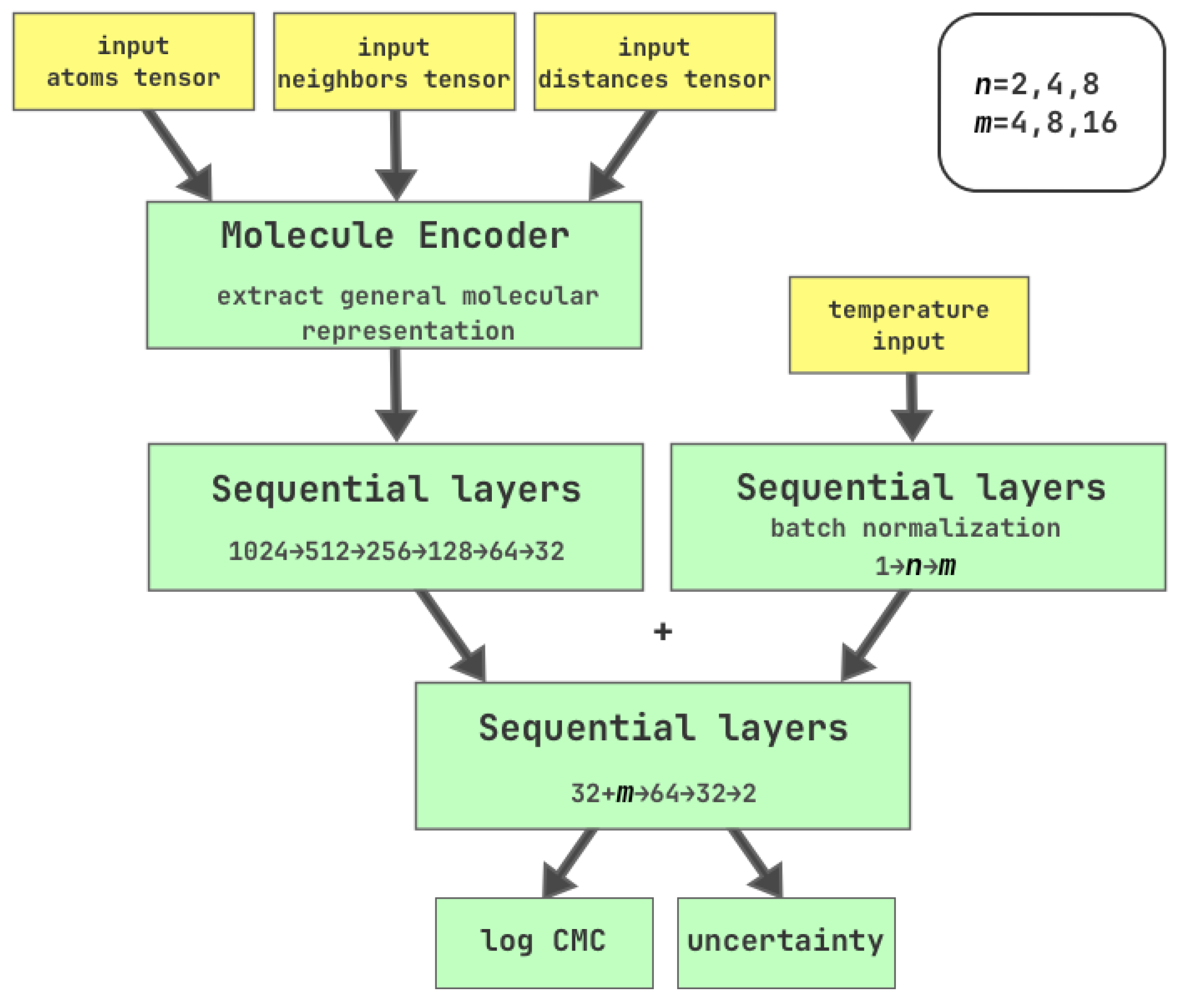
Figure 2.
The distribution of temperature in the final dataset excluding the external test set. The Y axis is displayed in logarithmic scale.
Figure 2.
The distribution of temperature in the final dataset excluding the external test set. The Y axis is displayed in logarithmic scale.
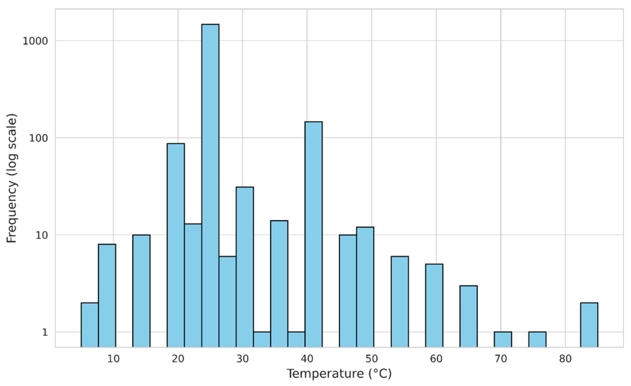
Figure 3.
Molecular mass distribution of the processed dataset before removal by 1300 g/mol upper bound.
Figure 3.
Molecular mass distribution of the processed dataset before removal by 1300 g/mol upper bound.
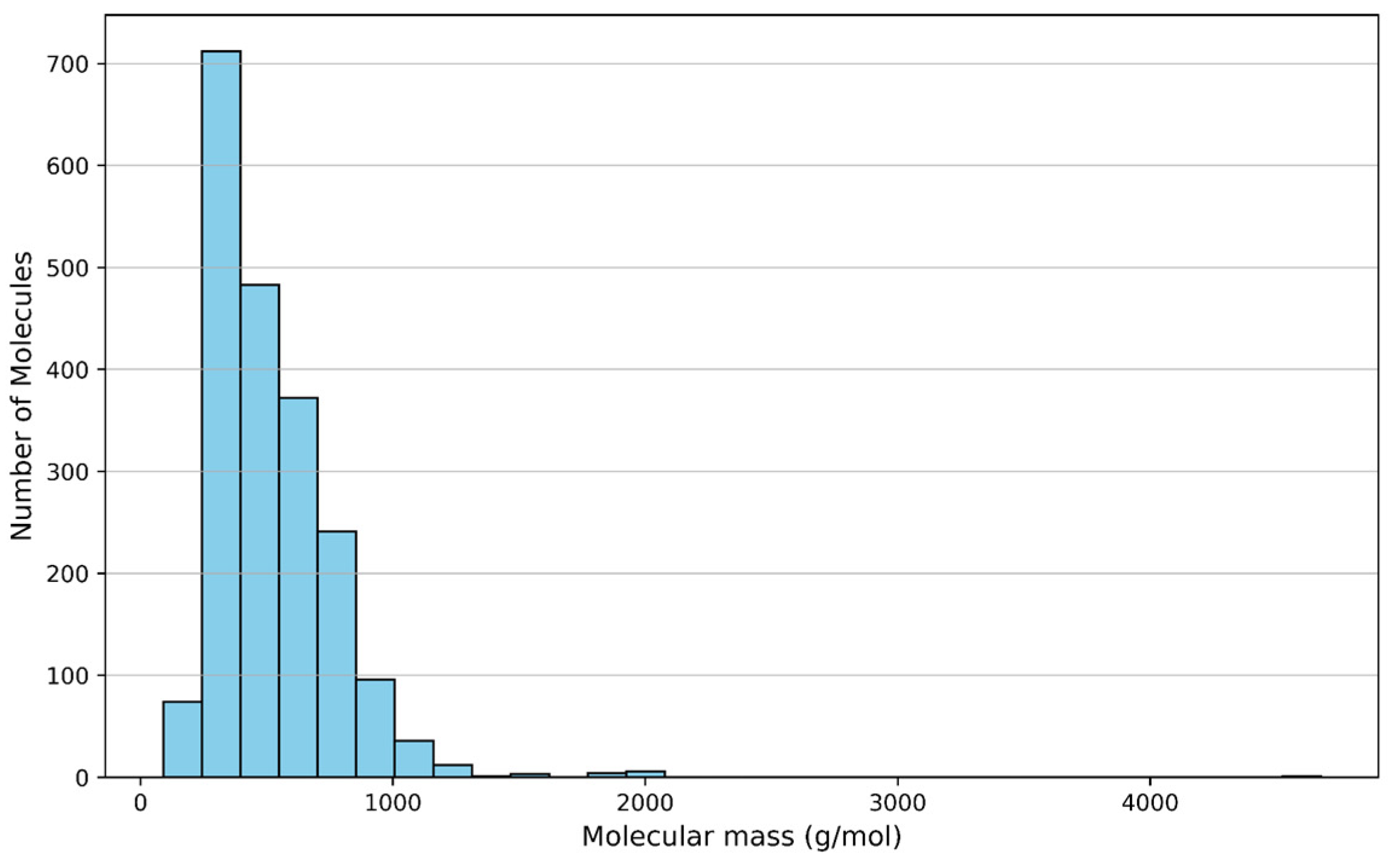
Figure 4.
Molecular mass distribution of the processed dataset after removing data points with molecular mass greater than 1300 g/mol.
Figure 4.
Molecular mass distribution of the processed dataset after removing data points with molecular mass greater than 1300 g/mol.
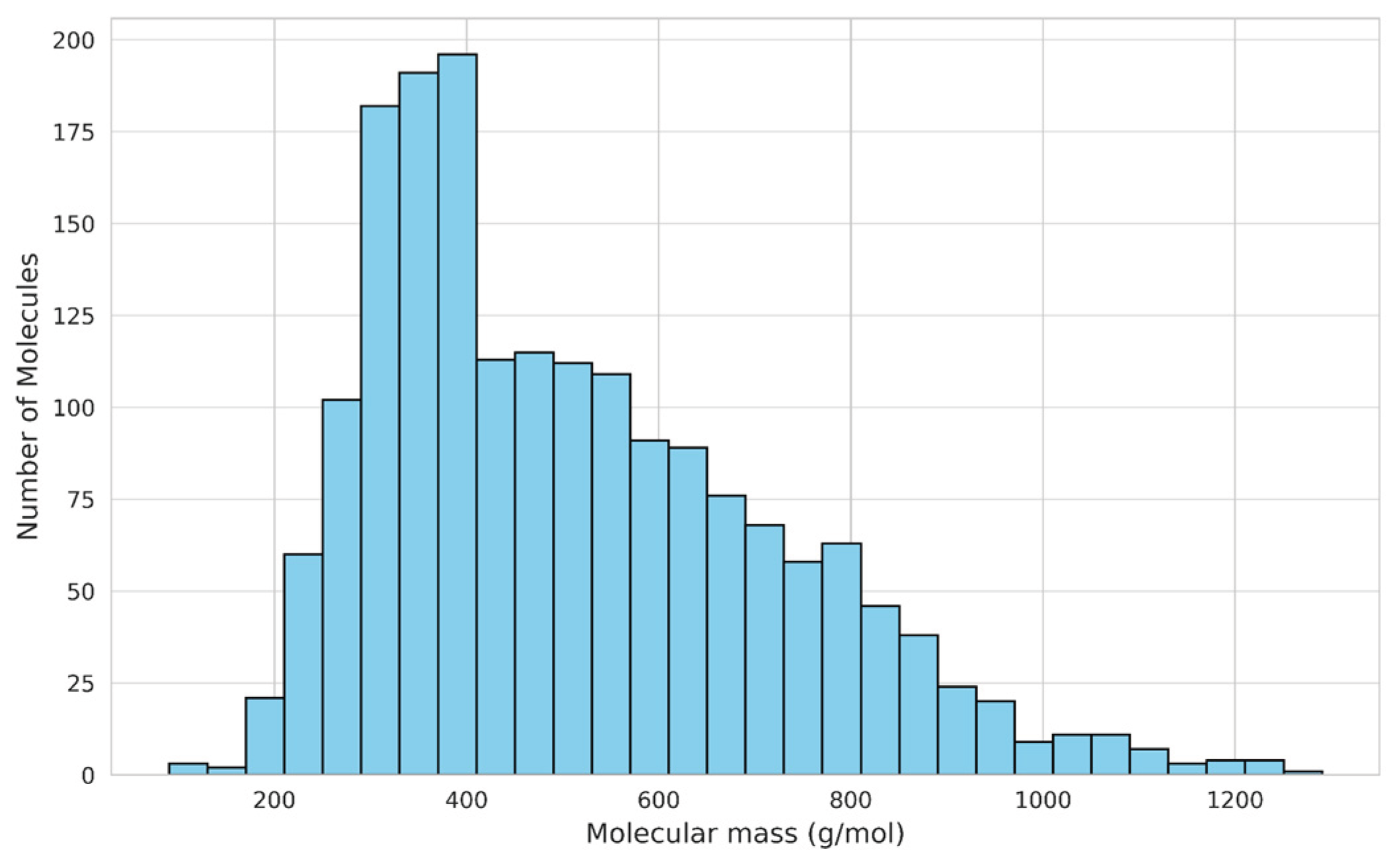
Figure 5.
The distribution of surfactant types in the processed dataset of 1829 data entries.
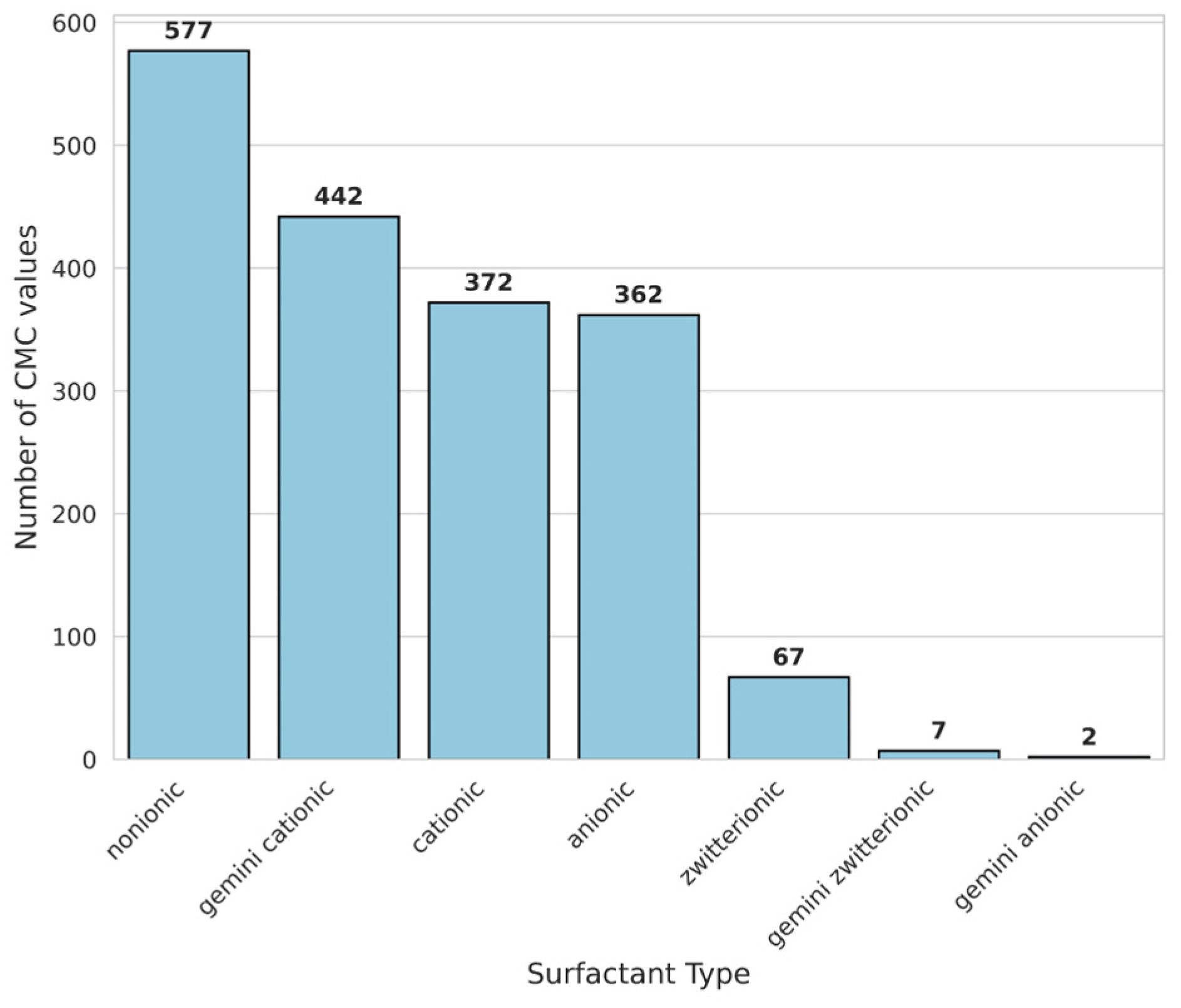
Figure 6.
Distribution of log CMC values for major surfactant categories in the processed dataset, with gemini surfactants of all charge types (cationic, anionic, zwitterionic) placed into a single "Gemini" category. The gray contour line represents the log CMC distribution of the complete dataset of 1829 data points for reference.
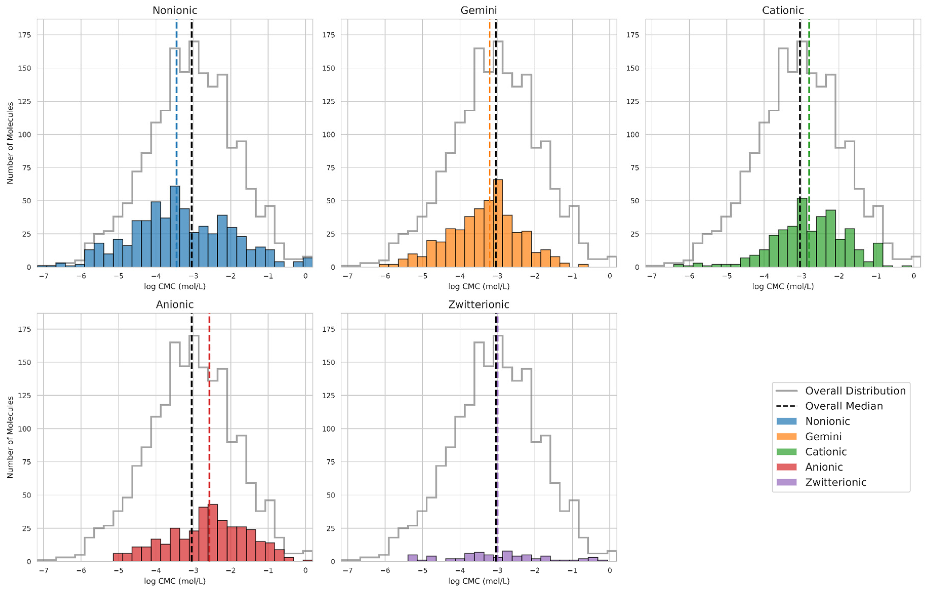
Figure 7.
Trained GNN models with different temperature MLP architecture performance metrics plots for internal test set: (a) RMSE and (b) R2. The best metric marked with green color – 1→4→8 temperature MLP architecture showed best results among the 3 explored architectures.
Figure 7.
Trained GNN models with different temperature MLP architecture performance metrics plots for internal test set: (a) RMSE and (b) R2. The best metric marked with green color – 1→4→8 temperature MLP architecture showed best results among the 3 explored architectures.
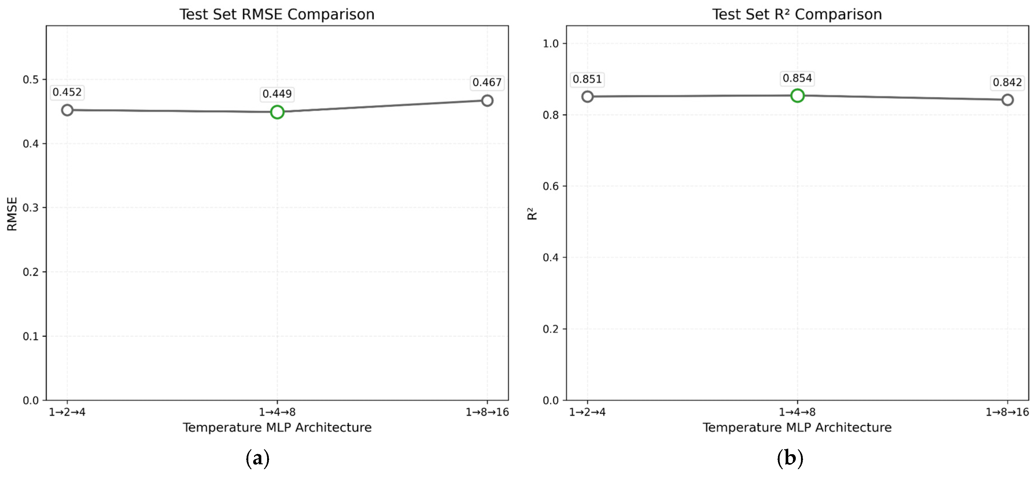
Figure 8.
Scatter plots of GNN-predicted versus true log CMC values: (a) Training set (1,829 data points) demonstrating strong model fit (R2 = 0.983); (b) Independent external test set (140 data points) confirming robust generalization capability (R2 = 0.892).
Figure 8.
Scatter plots of GNN-predicted versus true log CMC values: (a) Training set (1,829 data points) demonstrating strong model fit (R2 = 0.983); (b) Independent external test set (140 data points) confirming robust generalization capability (R2 = 0.892).
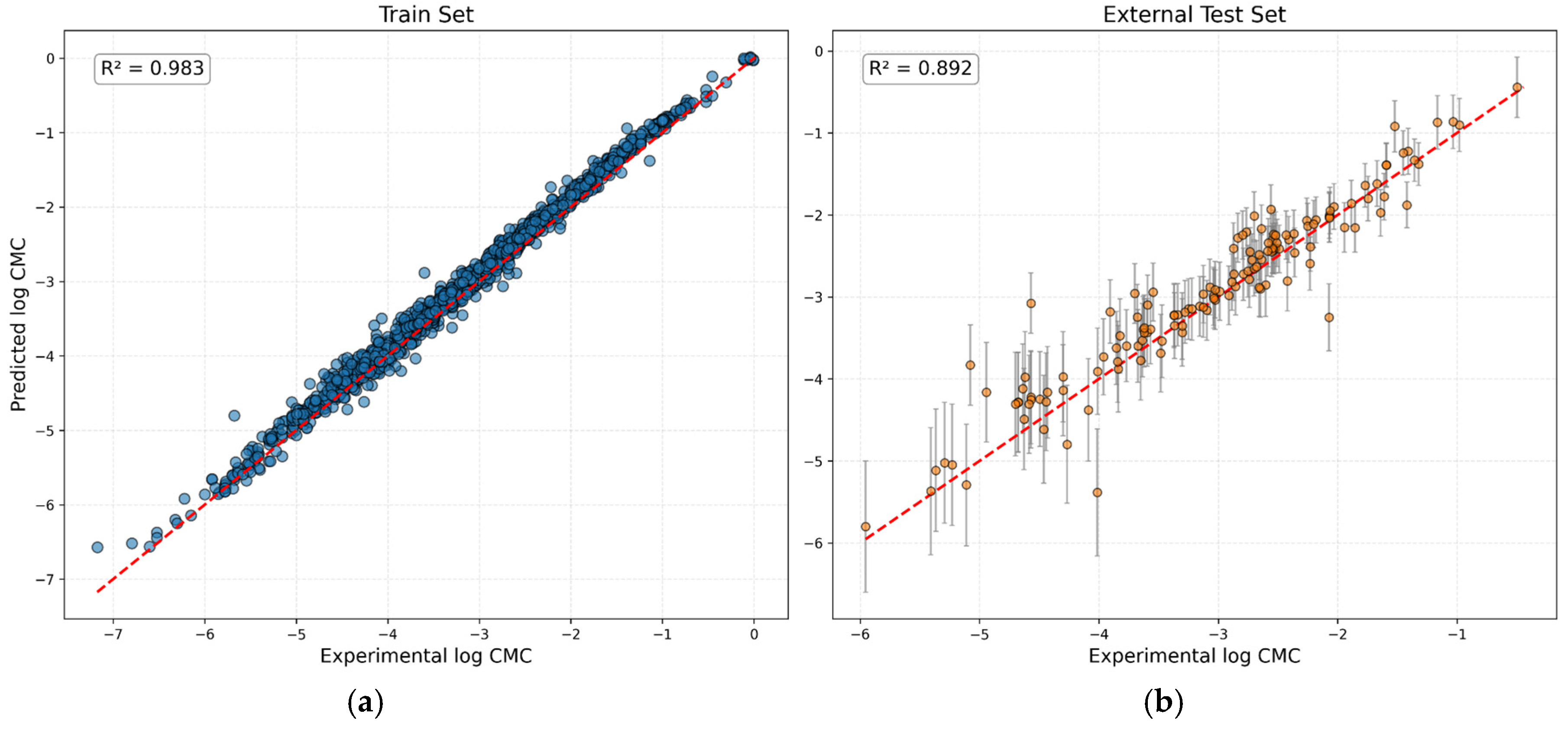
Figure 9.
Uncertainty and absolute prediction error correlation graph (Pearson correlation coefficient 0.2046, a = 0.3877, b = 0.0908).
Figure 9.
Uncertainty and absolute prediction error correlation graph (Pearson correlation coefficient 0.2046, a = 0.3877, b = 0.0908).
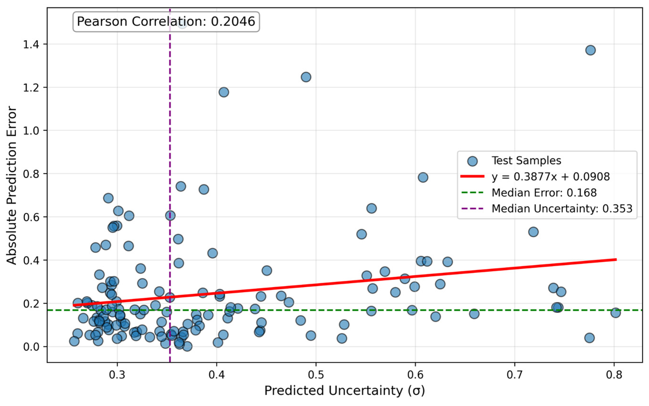

Table 1.
Performance metrics on the external test set (Hodl et al. [25] test set) for optimized fingerprint-based models.
Table 1.
Performance metrics on the external test set (Hodl et al. [25] test set) for optimized fingerprint-based models.
| Models | Parameters | R2 | MAE | MSE | RMSE |
| RF | minPath=2, maxPath=12, fpSize=4096 | 0,756 | 0,363 | 0,280 | 0,529 |
| XGB | minPath=2, maxPath=12, fpSize=4096 | 0,764 | 0,372 | 0,271 | 0,520 |
Table 2.
Performance metrics on the external test set (Hodl et al. [25]) for the trained GNN model and Hodl et al. model for comparison.
Table 2.
Performance metrics on the external test set (Hodl et al. [25]) for the trained GNN model and Hodl et al. model for comparison.
| Models | Parameters | R2 | MAE | MSE | RMSE |
| Hodl et al. model (SurfPro, 2025) | Training set: 1395 points Test set: 140 points Model: single property AttentiveFP GNN Temperature range: 20-40 °C MM limit: 4672 g/mol (≥2000) |
– | 0,241 | – | 0,365 |
| Our GNN Model | Training set: 1829 points Test set: 140 points Model: GNN (log CMC&uncertainty output) Temperature range: 5-85 °C MM limit: 1300 g/mol |
0,892 | 0,244 | 0,124 | 0,352 |
Disclaimer/Publisher’s Note: The statements, opinions and data contained in all publications are solely those of the individual author(s) and contributor(s) and not of MDPI and/or the editor(s). MDPI and/or the editor(s) disclaim responsibility for any injury to people or property resulting from any ideas, methods, instructions or products referred to in the content. |
© 2025 by the authors. Licensee MDPI, Basel, Switzerland. This article is an open access article distributed under the terms and conditions of the Creative Commons Attribution (CC BY) license (http://creativecommons.org/licenses/by/4.0/).
Copyright: This open access article is published under a Creative Commons CC BY 4.0 license, which permit the free download, distribution, and reuse, provided that the author and preprint are cited in any reuse.


