
Submitted:
05 December 2025
Posted:
08 December 2025
You are already at the latest version
Abstract
Since 2014, the Mexican Caribbean has faced an ecological and socio-economic crisis due to massive coastal landings of pelagic sargassum. This study presents a comprehensive methodology for sargassum detection using Machine Learning (ML) models applied to imagery from a coastal video monitoring station (EVMC). Three machine learning techniques were implemented to classify sargassum on sand and water, Support Vector Machines (SVM), Random Forest (RF), and a Multi-Layer Perceptron (MLP) Artificial Neural Network. The performance of these ground-based models was then compared against sargassum detections from Sentinel-2 satellite data using the Floating Algae Index (FAI) and the Normalized Difference Vegetation Index (NDVI). The results demonstrated high efficacy, with the MLP model proving most effective for detecting sargassum on sand with a F1-score > 0.86, whilst the Random Forest model performing best in water with a F1-score > 0.75. A significant positive correlation was found between the video-based detections and indices derived from satellite data, with NDVI showing a consistently stronger correlation in both environments. This study validates coastal video monitoring as a reliable tool for local sargassum quantification and suggests that fusing this high-resolution ground data with wide-area satellite imagery offers a promising path toward a more accurate and comprehensive sargassum monitoring system.
Keywords:
sargassum
; remote sensing
; machine learning
; Sentinel-2
; coastal monitoring
1. Introduction
Pelagic sargassum is a genus of macroalgae, commonly appearing in brown or green colors. Its defining biological feature is the presence of small, oxygen-filled vesicles called pneumatocysts, which act as flotation devices, allowing the algae to remain on the ocean’s surface [1]. The two primary species that constitute these massive floating mats are Sargassum natans and Sargassum fluitans.
Historically, sargassum was thought to originate and be concentrated almost exclusively within the Sargasso Sea, a vast region within the North Atlantic Subtropical Gyre [2,3]. However, since 2011, unprecedented and massive influxes of sargassum have inundated the coastlines of the central Atlantic and the Caribbean Sea, prompting scientific investigation into new sources [4,5].
Through a combination of satellite imagery, numerical models, and morphological analysis, researchers have identified two new major regions of origin: the North Equatorial Recirculation Region (NERR) and the vast expanse now known as the Great Atlantic Sargassum Belt (GASB) [4,6,7].
Several theories have been proposed to explain this dramatic increase in sargassum biomass. The most widely accepted theory points to eutrophication—an enrichment of water with nutrients that fuels explosive algal growth [8]. This nutrient overload is primarily attributed to increased discharge from major river systems, including the Amazon, Orinoco, and Congo rivers, which carry excess nitrogen and phosphorus linked to regional deforestation and changes in land use [9,10].
Monitoring a large-scale, dynamic phenomenon like sargassum blooms requires a perspective that must be addressed with innovative solutions. Satellite technology offered the first scalable solution for tracking sargassum across vast ocean basins. However, this approach has inherent limitations, particularly for coastal monitoring, which has driven a continuous cycle of innovation to develop more accurate and timely detection methods.
The primary scientific principle underpinning sargassum detection appling satellite data is a spectral phenomenon known as the "red edge." This refers to the sharp increase in light reflectance that occurs when moving from the red portion of the visible spectrum, around 680 nm, to the near-infrared (NIR) spectrum located in the interval of 700-730 nm. This signature is characteristic of healthy vegetation; chlorophyll strongly absorbs red light for photosynthesis, while the cellular structure of leaves strongly reflects NIR light. As floating algae, sargassum exhibits this same spectral behavior, making it distinguishable from the surrounding water from space [6].
Building on the red edge principle, scientists have developed several spectral indices to automate and quantify the detection of floating vegetation. Pioneering work in [11], first applied this principle to sargassum using imagery from the MERIS sensor, and the same research group later used the Maximum Chlorophyll Index (MCI) to identify the new sargassum accumulation regions in the Atlantic [6]. A key advancement came with the FAI, developed in [12], which refined detection by incorporating the short-wave infrared (SWIR) band to help differentiate floating matter from water.
Despite their utility for large-scale tracking, traditional satellite imagery and spectral indices face significant limitations, especially for critical coastal monitoring. Main difficulties at using only satellite imagery are the followings:
- Resolution Challenges: Both spatial and temporal resolution are major constraints.
- Spatial Resolution: Medium-resolution sensors cannot detect smaller sargassum patches, leading to a significant underestimation of the total quantity present [13].
- Temporal Resolution: Most freely available satellite sensors have revisit times of several days, making daily monitoring impossible [14].
- Atmospheric and Environmental Interference: The quality and usability of satellite images are frequently compromised by factors such as clouds, cloud shadows, and sun glint, which can obscure sargassum or be misclassified [15].
- Cost and Accessibility: While very high-resolution commercial satellites can overcome some resolution challenges, their high cost and restricted data access make them unsustainable for the long-term, continuous monitoring required for effective management [16].
- Spectral Confusion (False Positives): The spectral signature of sargassum is not unique. Other floating materials can mimic its reflectance pattern, leading to false positives. These include other types of marine vegetation (Trichodesmium, Syringodium), marine debris, and emulsified oil [17]. This problem is amplified in shallow coastal waters, where suspended particles interfere with the light signal, making near-shore detection particularly difficult and unreliable [18].
Machine Learning encompasses a set of computational procedures that learn to identify patterns within data to classify observations or make predictions [19]. The first published application of ML used a RF algorithm with Landsat 8 images [20]. Other traditional ML models, such as SVM and Gentle Boosting, have also been successfully applied [21]. More recently, deep learning—a subset of ML using neural networks—has shown significant promise. Models like ERisnet [22] and UNet [18] can process multiple data features (e.g., spectral bands, textures, locations) simultaneously, leading to highly accurate and nuanced detections.
The usage of fixed cameras installed on coastlines technically known as Coastal Video Monitoring Stations (EVMC) allows capturing high-frequency photographs of beaches. Previously, [15] successfully used convolutional neural networks on EVMC images for detection, while [23] used data from the same station in Puerto Morelos to study sargassum arrival dynamics.
Alternatively, the Citizen Science and Social Media Photographs from public participants are becoming a valuable data source. Programs like "Collective View" and "Sargassum Watch," along with images from social media platforms, are being used to train neural networks that can detect sargassum presence and even quantify its abundance [24] [25]. This leverages the power of distributed sensing, transforming passive observers into an active data collection network.
The preceding analysis reveals that while significant progress has been made, both traditional and advanced sargassum detection methods have distinct limitations. To overcome these challenges, this proposal outlines a novel, integrated approach that synergizes the strengths of large-scale satellite monitoring with high-resolution, ground-based photography, validated through a rigorous machine learning framework.
Even though others works have used EVMC imagery, this research will be the first to present a robust, automated methodology and, critically, to formally validate its performance against established satellite remote sensing indices. This cross-validation is the crucial missing step required to integrate high-frequency local data into the broader, basin-scale monitoring framework, thereby creating a truly holistic observation system.
The remainder of this paper is organized as follows: Section 2 presents the study area for sargasumm detection, data acquisition and ML processing techniques that is integrated in a novel multi-stage methodology through EVMC and satellite sources. Section 3 describes the performance of the machine learning models implemented for sargassum detection both on sand and water. Finally, Section 4 concludes this work and provides suggestions for future research directions.
2. Materials and Methods
The methodological framework for this study is structured into three principal phases, designed to systematically develop, apply, and compare two distinct sargassum detection approaches. This structure ensures a comprehensive evaluation of both a localized, high-frequency method and a broad-scale, lower-frequency method. The three core components of the methodology are:
- Sargassum Detection using EVMC Photographs: Development of a multi-stage machine learning pipeline to detect sargassum in ground-based coastal imagery.
- Sargassum Detection using Satellite Imagery: Application of established spectral indices to Sentinel-2 data to generate time series of sargassum presence.
- Comparative Time Series Analysis: A quantitative and qualitative comparison of the time-series data derived from both sources to assess their consistency, identify patterns, and evaluate their respective strengths.
This structured approach facilitates a direct comparison between the two methodologies, leading to a better understanding of their performance in monitoring sargassum dynamics.
2.1. Study Area
The study was conducted on the beach fronting the Unidad Académica de Sistemas Arrecifales of the Universidad Nacional Autónoma de México (UNAM), located at coordinates 20.8686193° N, -86.8682847° E in Puerto Morelos, Quintana Roo, Mexico as shown in Figure 1. As a key tourist destination, the economy of this region is highly vulnerable to sargassum influxes. Its geographic location places it directly in the transport pathway of the Yucatan Current, making it a frequent recipient of massive sargassum landings originating from the tropical Atlantic.
2.2. Coastal Video Monitoring Station (EVMC) Data
Coastal Video Monitoring Stations have been essential tools for investigating nearshore processes and analyzing their spatiotemporal dynamics (Holland et al., 1997; Holman and Stanley, 2007). In the context of Sargassum monitoring, these systems are particularly valuable, as they enable the continuous observation of massive Sargassum beaching events through the constant acquisition of imagery. The systems typically consist of a network of cameras installed at elevated sites near the coastline, capturing images at regular intervals and connected to an online server, which facilitates continuous data acquisition and storage (Berriel-Bueno, 2018). This uninterrupted image collection makes it possible to document and analyze the dynamic changes occurring within the coastal environment, providing a detailed and temporally consistent description of shoreline variability (Jóia Santos et al., 2020). A sample photography shown the coast with sargassum along the border of the beach is shown in Figure 2.
The procedure for getting the images from EVMC for this work is as follows:
- Source: The images were captured by two Allied Vision Stingray cameras installed by the Laboratorio de Ingeniería y Procesos Costeros (UNAM).
- Specifications: The cameras were installed at a height of 15 meters and captured images with a resolution of 960 x 1280 pixels.
- Collection Protocol: Images were captured hourly during daylight hours.
- Study Period and Dataset Size: The study period spanned from June 6, 2016, to May 20, 2021, yielding an initial dataset of approximately 30,000 images.
2.3. Satellite Data
Satellite imagery and spectral indices have been fundamental in enhancing the understanding of Sargassum dynamics, as they enable its detection across remote oceanic regions. However, these datasets present inherent limitations related to their temporal and spatial resolution [14] (Rodríguez-Martínez et al., 2022), as well as atmospheric factors intrinsic to satellite observations—such as shadows, sun glint, and cloud cover—that can significantly affect the accuracy of Sargassum detection.
The procedure for getting the images from satellite data for this work is as follows:
- Source: Imagery was acquired from the European Space Agency’s (ESA) Sentinel-2 mission via the Google Earth Engine (GEE) platform.
- Product Level: Level-1C products, providing Top-of-Atmosphere (TOA) reflectance, were used.
- Filters and Dataset Size: A cloud cover filter of less than 10% was applied, resulting in a final dataset of 251 images over the same study period.
- Spectral Bands: The analysis utilized the Blue, Green, Red, and Near-Infrared (NIR) bands, all at 10-meter spatial resolution.
A sample photography from Sentinel-2 constellation capturing the coast with sargassum along the border of the beach is shown in Figure 3.
2.4. EVMC Image Preprocessing and Feature Engineering
Detecting sargassum from the EVMC photographs presented significant challenges due to variable lighting, oblique camera angles, and complex scenes containing multiple elements (sand, water, vegetation, buildings). In order to overcome these issues, a sophisticated, multi-step machine learning pipeline was developed. The process involved the following key stages:
- (i)
- Optimal Photograph Selection
- (ii)
- Region of Interest (ROI) Masking
- (iii)
- Training Dataset Creation and Labeling
- (iv)
- Feature Analysis
- (v)
- Model Training and Prediction
Four distinct machine learning models were trained and evaluated for their ability to classify pixels as either sargassum or non-sargassum: SVM with both linear and Radial Basis Function (RBF) kernels, MLP, RF.
2.4.1. Photograph Selection and Preprocessing
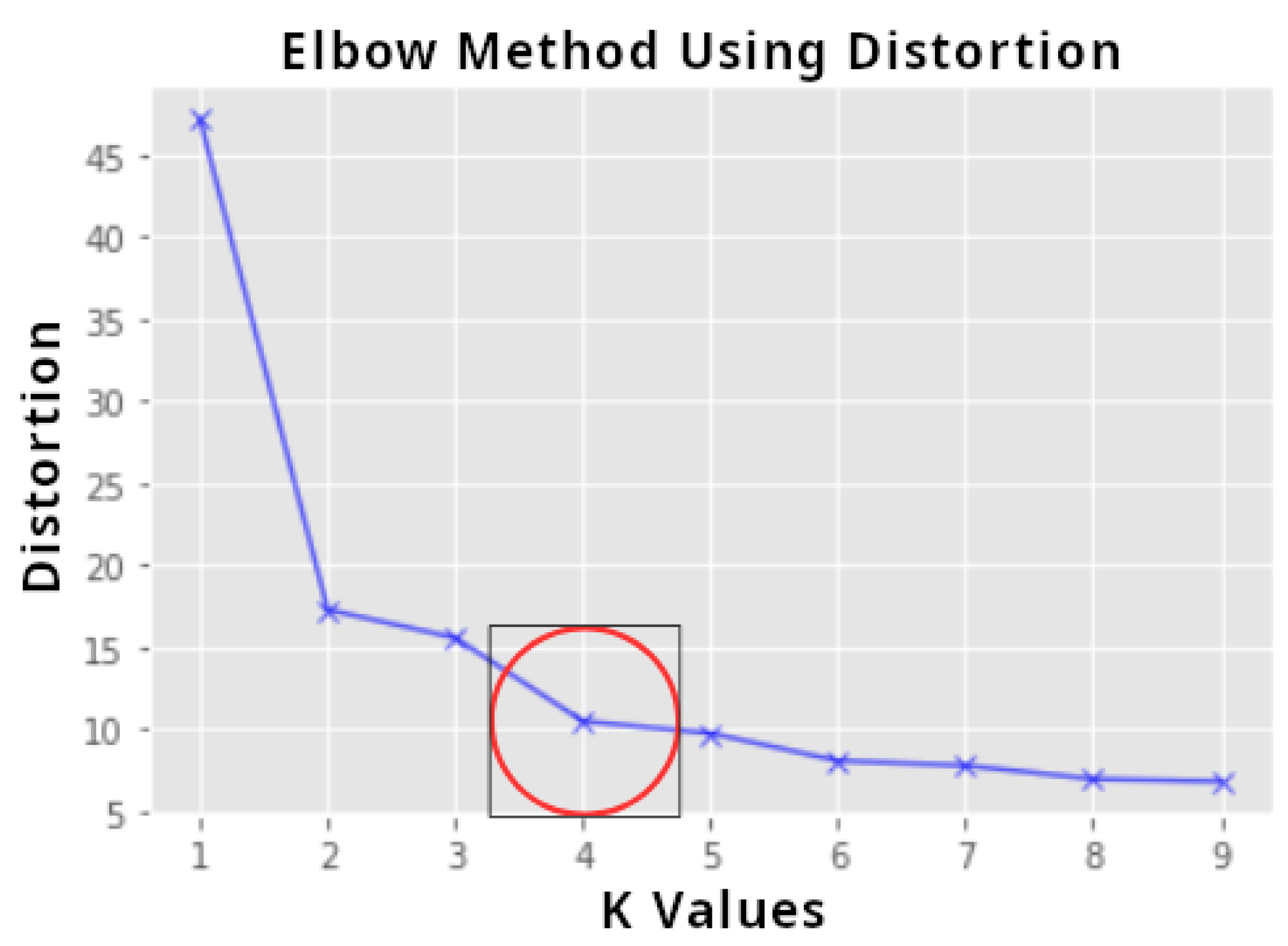
A primary challenge with the hourly EVMC photographs was the significant intra-day variability in lighting, which produced a dataset containing images unsuitable for analysis. Some photographs taken in the early morning were too dark to discern any features, while others were compromised by significant sun glare (specular reflection) on the water surface. These confounding factors make automated feature extraction unreliable. This step was designed as a critical solution to isolate a subset of images free from these issues. To systematically identify images with optimal illumination, the K-means clustering algorithm was implemented. Each photograph was represented by a six-dimensional vector of its average color components: (R, G, B) from the RGB color space and (H, S, V) from the HSV color space. Both the elbow method and silhouette coefficient analysis were used to determine the optimal number of clusters (K), with both methods indicating that K=4 was the most appropriate value for partitioning the dataset.
Figure 4.
Distortion curve as a function of the number of K clusters, using RGB and HSV color features.
Figure 4.
Distortion curve as a function of the number of K clusters, using RGB and HSV color features.
To create a consistent daily record, a single representative photograph for each day was generated by averaging all photos taken within this three-hour window. This consolidation process reduced the dataset from ≈30,000 initial images to the final set of 1643 images used for model training and prediction.
2.4.2. Region of Interest Masking
The region of interest for Sand was extracted through the MOG2 Background Subtraction algorithm [26], for the purpose of distinguish the static background from the dynamic foreground. A critical consideration was the significant change to the beach profile caused by Hurricane Zeta in October 2020. To account for this, two separate masks were created: one for the pre-hurricane period and another for the post-hurricane period.
On the other hand, the same algorithm proved ineffective for the water surface, as the dynamic nature of waves and floating sargassum prevented the algorithm from establishing a stable background model. An alternative method was developed: a composite mask was created by summing all the manually labeled sargassum detection zones from the training images. This approach effectively defined the geographic areas within the image where sargassum was most commonly observed.
2.4.3. Training Dataset
The procedure for building the training and testing sets for each model, one representative image was selected for each month of the study period, along with twelve additional random images, resulting a total of 72 training images. A separate set of 20 images was reserved for testing. The manual labeling was performed, where binary masks were created by coloring sargassum pixels white and all non-sargassum pixels black. To prevent class imbalance, where one class (e.g., non-sargassum) vastly outnumbers the other, a pixel balancing strategy was employed. For each labeled image, the class with the fewer number of pixels determined the sample size, and an equal number of pixels was then randomly sampled from the more abundant class.
2.4.4. Feature Selection and Analysis
Sargassum detection was performed at the pixel level. For each pixel within the defined ROI, a vector of six color features was extracted to serve as input for the machine learning models:
- RGB: Red, Green, Blue
- HSV: Hue, Saturation, Value
A feature importance analysis was conducted using decision trees with the Gini impurity criterion in order to understand which of these features were most influential. This helped identify the most discriminating features for model construction and improved the interpretation of the results. Validation of the analysis was conducted using histograms for all six features were generated from a sample of 200,000 pixels for each of the primary scene elements (sand, vegetation, water, sargassum on sand, and sargassum in water). This allowed for a visual inspection and comparison of their distinct color distributions.
2.4.5. Model Training and Time Series Generation
Four machine learning algorithms were trained for both the Sand and Water detection tasks using the labeled training data. The key hyperparameters for each model were as follows:
- Random Forest: 100 trees, 3 features per tree, Gini Impurity criterion.
- Support Vector Machine: Linear Kernel: Hinge loss function, max 1000 iterations.
- RBF Kernel: Gamma value set to scale, which is calculated as 1 / (number of features x varianza of data).
- Multilayer Perceptron: An architecture consisting of an input layer, two hidden layers with eight neurons each, and an output layer. The model used a ReLU activation function, and the ADAM optimizer for weight optimization.
After training, the models were applied to the full dataset of 1643 daily averaged photographs to predict the presence of sargassum. This process generated a final time series for each algorithm and medium (sand/water). Each data point in the series represents the daily sargassum pixel density, defined as the total count of pixels classified as sargassum divided by the total number of pixels in the corresponding ROI. It is important to acknowledge a key limitation of this method. As noted in [27], without extrinsic camera calibration and image projection to correct for perspective distortion, the pixel count represents an approximate measure of sargassum quantity and cannot be directly translated into a real-world area unit (e.g., square meters).
2.5. Comparative Time Series Analysis
The primary goal of this final phase was to quantitatively and qualitatively compare the time series generated from the EVMC machine learning models and the satellite-derived spectral indices. This comparison aimed to assess their consistency, identify shared patterns in sargassum accumulation, and evaluate their complementary strengths. Before comparison, all time series underwent several preprocessing steps:
- Normalization: Standard normalization (z-score) was applied to scale all data to a mean of zero and a unit variance, allowing for direct comparison of series with different native scales.
- Smoothing: The Savitzky-Golay filter was used to reduce high-frequency noise. This noise can originate from factors like intermittent cloud cover in satellite data or poor weather and camera lens issues (e.g., water droplets) in the EVMC imagery. This technique is well-established for smoothing spectral index time series [28] Huang et al., 2021).
A significant challenge was comparing time series of unequal lengths (1643 EVMC data points versus 251 satellite data points). Two adaptation strategies were used to address this:
- The common dates method: New, shorter series were created containing data only from dates that were present in both the EVMC and satellite datasets, allowing for direct, day-to-day comparison.
- The monthly averages method: Monthly average values were calculated for all series, creating datasets of equal length that capture lower-frequency trends.
Several similarity and correlation metrics were employed to evaluate the relationships between the series:
- Correlation Coefficients: Both Pearson and Spearman coefficients were calculated, with the appropriate choice informed by examining scatter plots of the data.
- Cross-Correlation: This method was used to evaluate the association between series at different time lags, helping to identify potential lead-lag relationships [29].
- Dynamic Time Warping (DTW): This algorithm measures the similarity between two temporal sequences that may vary in speed or time [30]. Unlike Pearson or Spearman correlation, which require series of equal length and assess linear or monotonic relationships, DTW is adept at finding underlying similarities between temporal patterns even when they are out of phase or stretched in time, making it particularly suitable for comparing the high frequency EVMC data with the sparser satellite acquisitions. It calculates a minimal cumulative distance score between the series.
Another study to investigate underlying patterns is a time series decomposition analysis using an additive model (series = trend + seasonality + noise). This separates each time series into its constituent components, enabling a direct comparison of the long term trends and seasonal patterns captured by the different detection methods.
Finally, as a qualitative validation step, the trends, peaks, and valleys observed in the generated time series were visually compared with the findings in [31]. That study monitored sargassum in the same region using Landsat 8 imagery with a mix of spectral indices NDVI, FAI, Soil Adjusted Vegetation Index (SAVI) and a Random Forest model, supplemented with sargassum removal reports from local hotels. This external comparison served to corroborate the patterns identified in this research.
This comprehensive approach, combining direct correlation, advanced similarity metrics, component decomposition, and external validation, provides a thorough evaluation of the two sargassum detection methodologies.
2.6. Satellite Image Processing
The analysis of the 251 preprocessed Sentinel-2 images was conducted entirely on the Google Earth Engine (GEE) platform. To detect sargassum presence, two well-established spectral indices were calculated for each image:
- Normalized Difference Vegetation Index (NDVI): Primarily used for detecting sargassum washed ashore on the beach.
- Floating Algae Index (FAI): Used for detecting floating sargassum mats in the water.
A custom JavaScript code was developed in the GEE code editor to automate the analysis pipeline. This script performed several key functions: it selected the required spectral bands (Blue, Green, Red, NIR), applied the mathematical operations to calculate the NDVI and FAI indices, filtered out pixels with over 10% cloud cover to ensure data quality, and generated two distinct time series. Each data point in these series represents the average index value (NDVI or FAI) within the defined ROI for a given date.
This rigorous methodology provides a robust framework for evaluating the performance of the ML models and understanding the relationship between ground-based and satellite-based sargassum detection systems.
3. Results
This section presents the quantitative findings of the study. It begins with an analysis of the most important color features for sargassum detection, followed by a comparative evaluation of the machine learning models’ performance in different coastal environments. The section concludes with the results of the time-series comparison between the ground-based video monitoring and satellite-based detection methods.
3.1. Feature Importance Analysis for Sargassum Detection
3.1.1. Key Features for Sargassum on Sand
For detecting sargassum on sand, the analysis sought to distinguish dry sargassum from sand and other terrestrial vegetation.
An analysis based on Gini impurity reduction in a decision-tree framework revealed that the most important features for detecting sargassum on sand were the Green and Red channels, followed by the Value component Figure 5.
Moreover, an analysis of feature histograms confirmed that RED and GREEN provides a clear separation in the statistical distributions of these features when comparing pixels of sargassum, sand, and terrestrial vegetation Figure 6.
3.1.2. Key Features for Sargassum on Water
Detecting sargassum in water requires separating its signature from the surrounding water, a task complicated by waves, turbidity, and reflections. For distinguishing sargassum in the water, the Hue feature was overwhelmingly the most important characteristic. The Blue channel was the second most important feature Figure 7.
Again, histogram analysis validated this result, showing a distinct distribution for the Hue value of sargassum pixels compared to water pixels, demonstrating its relevance in separating both Figure 8.
3.2. Performance of Machine Learning Models
The regions of sargassum detected over the sand for the four machine learning models are marked in red color as show in Figure 9.
Oh the other hand, the regions of sargassum detected over the water are shown in Figure 10.
The performance of these models for pixel-level classification was evaluated using 10-fold cross-validation. The F1-score and accuracy metrics are summarized in Table 1 for the sand and water environments.
3.2.1. Model Performance for Sargassum on Sand
The models were trained and tested on image data of sargassum accumulated on the beach. The performance metrics presented below apply specifically to this on-sand dataset.
The MLP Neural Network emerged as the top-performing model, achieving the highest F1 score (0.8898) and accuracy (0.8831) on the test set. Three of the four models; RF, MLP NN, and SVM RBF; demonstrated robust performance, with F1 and accuracy scores consistently above 0.85. A clear trade-off exists between performance and computational cost. Despite this, MLP was the slowest to train (315.24 s), whereas the linear SVM was the fastest but delivered the lowest performance. The SVM RBF, while highly accurate, was impractical for high-throughput applications due to its exceptionally slow prediction time (870.76 s). In order to validate the need for environment-specific models, a cross-environment test was conducted by applying these sand-trained models to in-water images. The results confirmed their non-transferability, as the F1 scores plummeted to a range of 0.4778 (SVM Linear) to 0.6125 (SVM RBF). Finally, a Dynamic Time Warping (DTW) analysis of the prediction time series in this models, revealed that the outputs from the RF and MLP were the most similar (distance of 0.512).
3.2.2. Model Performance for Sargassum on Water
The same set of algorithms was evaluated for the more complex task of detecting sargassum floating in water. The metrics below apply to the in-water dataset.

Table 2.
Performance metrics ML algorithms for sargassum detection on sand.
| Model | Metric | Test Set Score |
Cross Validation Average |
Training Time (s) |
Prediction Time (s) |
|---|---|---|---|---|---|
| Random Forest | F1-score | 0.7299 | 0.7599 | 291.48 | 22.37 |
| Accuracy | 0.7695 | 0.8133 | |||
| Multilayer Perceptron | F1-score | 0.7283 | 0.7490 | 330.10 | 3.94 |
| Accuracy | 0.7688 | 0.8059 | |||
| SVM RFB | F1-score | 0.7295 | 0.7598 | 637.54 | 574.63 |
| Accuracy | 0.7691 | 0.8087 | |||
| SVM Lineal | F1-score | 0.6712 | 0.6123 | 255.29 | 1.82 |
| Accuracy | 0.6913 | 0.7053 |
The Random Forest model was the best for in-water detection, though its performance was very closely matched by the MLP and SVM RBF. All three top models achieved F1 and accuracy scores above 0.70, with the lower overall scores confirming that in-water detection is a more challenging classification task, a difficulty often apparent even to the human eye.
Computationally, the linear SVM was again the fastest but least accurate, while the SVM RBF was exceptionally slow, particularly in prediction. The cross-environment test, applying water-trained models to sand images, again reinforced the need for specialized models; while the RF model performed reasonably (accuracy > 0.83), the performance reduction was significant enough to justify a dedicated on-sand model.
The DTW analysis echoed the over sand findings, with the RF and MLP models producing the most similar time series and the linear SVM generating a significantly different output.
Having established the superior predictive power of the MLP and RF models for their respective domains, the critical next step is to validate their real-world performance by correlating their temporal outputs against established satellite based spectral indices.
3.3. Time Series Analysis
The normalized time series of the number of pixels detected as Sargassum across the four learning models are shown for arena (Figure 11) and water (Figure 12).It is observed that the predictions are remarkably similar to one another. The only time series that appears slightly different corresponds to the one generated by the SVM model with a linear kernel.
3.3.1. Time Series for Sargassum on Sand
The time series generated by the best ML model on sand (MLP) was compared with NDVI and FAI data derived from Sentinel-2 satellite imagery.
Statistical Correlation: Given the monotonic but not strictly linear relationship observed in scatter plots, the Spearman rank correlation () was used. The analysis revealed a moderate positive correlation () between the MLP time series and the NDVI series for days with corresponding data. In contrast, the FAI series showed a weak correlation (), an expected outcome as FAI is designed for detecting floating vegetation in water, not on land. Cross-correlation analysis confirmed a direct temporal correspondence, with the strongest relationship found at a lag of zero.
Visual Analysis: Inspection of the time series plots showed periods of strong agreement, particularly in identifying the high-sargassum seasons of mid-2018 and mid-2019, as well as periods with little to no sargassum. Disagreements were noted in specific periods, potentially attributable to factors like satellite image errors (e.g., residual cloud cover) or different algal conditions not captured equally by the ground camera and the spectral indices.
Time Series Decomposition: A decomposition of the 2018–2020 time series using an annual window (62 data points) showed that while all series exhibited a clear annual seasonality, their long-term trends differed. Both spectral indices showed a decreasing trend over the period, whereas the MLP model identified 2019 as the peak year. It is critical to note that this trend is specific to the 2018-2020 period and does not necessarily represent a long-term decline in sargassum events.
3.3.2. Time Series for Sargassum in Water (Random Forest Model)
Similarly, the time series from the best model on water (RF), was correlated against the spectral indices.
Statistical Correlation: As scatter plots indicated a stronger linear trend, the Pearson correlation coefficient (r) was deemed appropriate. The RF time series demonstrated a strong positive correlation with both NDVI () and FAI () for common dates images. The stronger correlation with FAI in this context is logical, given its specific design for detecting floating algae. Cross-correlation analysis again found the maximum correlation at a temporal lag of zero, indicating the ground and satellite detection were synchronized.
Visual Analysis: The time series plots showed strong consensus during periods of both high and low sargassum levels. Some discrepancies appeared to coincide with potential artifacts in the satellite data, such as residual clouds that could be misread by the spectral indices.
Time Series Decomposition: Decomposition for the 2018–2020 period, using an annual window of 62 data points, revealed a high degree of consistency. All three series (RF, NDVI, and FAI) showed a similar decreasing trend over the three years and a distinct annual seasonality, with sargassum presence peaking in the summer months. As with the on-sand analysis, this observed trend applies only to the study period.
The Table 3 summarize the coefficients correlation previously described and that supports the validation of the corresponding ML model.
3.3.3. External Validation
This section compares the generated sargassum time series with the results from [31]. In that work, data sources, Landsat 8 satellite imagery and sargassum removal reports from local hotels to analyze sargassum trends in the same geographic area of Puerto Morelos.
While both studies identified 2018 and 2019 as years with significant sargassum events and observed a near-total absence from late 2019 to mid-2020, notable differences were also present. The observed discrepancies, such as the different peak month in 2019 (July in this study vs. April in [31]), are best explained by the fundamental difference in observational scale. In this work, high-frequency, fixed-point camera methodology captures hyper-local accumulation events with high granularity, registering more frequent high-sargassum periods. In contrast, the regional scope in [31] using lower-frequency satellite data and aggregated reports, provides a broader, spatially averaged perspective.
4. Discussion
This section analyzes the implications of the findings on the results, beginning with an interpretation of the performance of the machine learning models and the critical role of specific color features in sargassum detection. It then critically evaluates the observed correlations between the ground-based and satellite monitoring systems, concluding with a discussion of the complementary strengths and weaknesses of each approach for a comprehensive monitoring strategy.
4.1. Interpreting Model Performance and Feature Importance
The superior performance of non-linear models like the MLP and Random Forest demonstrates that the relationship between pixel color values and the presence of sargassum is complex. The data is not separable by a simple linear boundary, which explains the significantly lower accuracy of the linear SVM model.
The analysis of feature importance provides valuable insights into the detection process. For sargassum on sand, the importance of the Green and Red channels is expected; the Green channel likely helps differentiate the brownish sargassum from green terrestrial vegetation at the back of the beach, while the Red channel captures the characteristic color of the algae itself. This aligns with the fundamental red edge principle, where the spectral contrast between red absorption and near-infrared reflectance is paramount, a phenomenon that remains influential even within the more limited RGB color space. In the water environment, the overwhelming importance of Hue highlights its effectiveness in capturing the subtle but consistent color difference between sargassum and the highly variable blue-green background of the sea. Hue isolates the color type, making it more robust against changes in lighting and water conditions compared to the combined RGB channels. The need for two separate models, one for sand and one for water, was justified by cross-prediction tests, which showed a significant drop in accuracy when a model trained for one environment was used to predict on the other.
4.2. Significance of the Correlation Between Ground and Satellite Data
The moderate/strong positive correlations between the EVMC-based ML detection and the Sentinel-2 satellite indices serve as a crucial validation. They confirm that the ground-based methodology is a legitimate approach for quantifying local sargassum abundance, as its outputs trend consistently with established, large-scale remote sensing indicators. The high correlation observed with NDVI in both sand and water environments is noteworthy. This suggests that NDVI is a robust and versatile index for detecting vegetative matter against varied backgrounds, including both sand and water. The performance of FAI, while strong in water, was weaker on sand, which is expected since the index was specifically designed to detect floating algae against a water baseline. Its slightly lower correlation in water compared to NDVI could be attributed to its known sensitivity to the environmental conditions characteristic of the near-shore study site, such as water turbidity and shallow depths, which can interfere with its signal.
4.3. Complementary Roles of EVMC and Satellite Monitoring Systems
This study clearly illustrates that EVMC and satellite systems are not competing technologies but rather highly complementary tools for sargassum monitoring. Each system possesses unique strengths that address the weaknesses of the other.
- EVMC System: The primary advantage of the EVMC system is its ability to provide high-resolution data, both spatially (pixel-level detail) and temporally (hourly images). This makes it ideal for accurate local quantification and management. It can provide precise, daily measurements of beached sargassum to inform cleanup logistics and assess coastal impact. However, its disadvantages include a limited spatial coverage that provides no early warning, vulnerability to local conditions like a dirty lens or adverse weather, and an intensive initial data processing and model training requirement.
- Satellite System: Their main advantage is its vast spatial coverage, enabling regional-scale monitoring and early warning. Satellites can track large sargassum blooms in the open ocean days or weeks before they make landfall, which is critical for forecasting and preparedness. Its key disadvantages are its lower resolution, which can lead to underestimation of sargassum volume; its susceptibility to cloud cover, which creates data gaps; and its reduced accuracy in the complex coastal zones where impacts are most severe.
Ultimately, an integrated system that leverages both technologies would be optimal. Satellites could provide the broad-scale forecasting needed for early warning, while EVMC systems would offer the high-resolution "ground-truth" data required to validate satellite detection, quantify the precise coastal impact, and guide local management responses.
This analysis underscores the potential of a multi-platform approach, leading to the final conclusions and future outlook of the study.
5. Conclusions
This study successfully developed, implemented, and validated a novel methodology for the automated detection and quantification of sargassum using ML models applied to coastal video monitoring imagery. Particularly non-linear models like Multi-Layer Perceptrons and Random Forests, can effectively and automatically detect sargassum on both sand and in near-shore waters from standard video monitoring stations with high accuracy.
The statistically significant positive correlations found between our ground-based detections and established satellite-derived indices (NDVI and FAI) from Sentinel-2 data confirm the viability and reliability of the EVMC-based approach for monitoring local sargassum dynamics. Both systems are not competitors but are highly complementary. An integrated strategy, combining the broad-scale predictive power of satellites with the high-resolution quantitative accuracy of coastal video stations, represents the most effective path forward for a comprehensive sargassum monitoring and management system.
Author Contributions
For this research the authors contributes as follows: Conceptualization, B.d.l.B.-B. and J.H.-B.; methodology, B.d.l.B.-B.; software, M.S.-S.; validation, O.S.-S. and J.H.-B.; formal analysis, B.d.l.B.-B., J.H.-B. and M.S.-S.; investigation, B.d.l.B.-B.,V.S.-C and O.S.-S.; resources, O.S.-S. and M.S.-S.; data curation, M.S.-S. and B.d.l.B.-B..; writing—original draft preparation, B.d.l.B.-B.,V.S.-C and J.H.-B.; writing—review and editing, O.S.-S., V.S.-C and J.H.-B.; visualization, M.S.-S. and B.d.l.B.-B..; supervision, B.d.l.B.-B. and J.H.-B.; project administration, M.S.-S. and B.d.l.B.-B.. All authors have read and agreed to the published version of the manuscript.
Funding
This research received no external funding. It was supported by the Secretaría de Ciencia, Humanidades, Tecnología e Innovación (SECIHTI) through the National Scholarships Program (Programa de Becas Nacionales).
Data Availability Statement
The satellite imagery used in this study was obtained from the European Space Agency and is publicly available. The fixed-camera images were provided by the Laboratorio de Ingeniería y Procesos Costeros de la Unidad Académica Sisal of the Instituto de Ingeniería de la UNAM, which is responsible for their maintenance and distribution. Contact information for the data providers can be shared by the authors upon request.
Acknowledgments
The authors would like to thank the Laboratorio Nacional de Geointeligencia (GeoInt) for the facilities provided to carry out this study. We also acknowledge the support of the Secretaría de Ciencia, Humanidades, Tecnología e Innovación (SECIHTI) through its scholarship program. Finally, we thank Dr. Tonatiuh Mendoza from the Laboratorio de Ingeniería y Procesos Costeros de la Unidad Académica Sisal of the Instituto de Ingeniería de la UNAM for providing the fixed-camera images used in this study.
Conflicts of Interest
The authors declare no conflicts of interest.
Abbreviations
The following abbreviations are used in this manuscript:
| ML | Machine Learning |
| SVM | Support Vector Machine |
| RF | Random Forest |
| MLP | Multi-Layer Perceptron |
| FAI | Floating Algae Index |
| NDVI | Normalized Difference Vegetation Index |
| NERR | North Equatorial Recirculation Reggion |
| GASB | Great Atlantic Sargassum Belt |
| NIR | Near infrared |
| SWIR | Short Wave Infrared |
| MCI | Maximum Chlorophyll Index |
| EVMC | Coastal Video Monitoring Stations |
| UNAM | Universidad Nacional Autónoma de México |
| GEE | Google Earth Engine |
| ROI | Region of Interest |
| RGB | Red, Green, Blue |
| HSV | Hue, Saturation, Value |
| DTW | Dynamic Time Warping |
References
- Council, S.A.F.M. Fishery management plan for pelagic sargassum habitat of the South Atlantic Region. Technical report; National Marine Fisheries Service, NOAA, 2002. [Google Scholar]
- Lapointe, B.E. A comparison of nutrient-limited productivity in Sargassum natans from neritic vs. oceanic waters of the western North Atlantic Ocean. Limnology and Oceanography 1995, 40, 625–633. [Google Scholar] [CrossRef]
- Gower, J.; King, S. Satellite images show the movement of floating Sargassum in the Gulf of Mexico and Atlantic Ocean. Nature Precedings 2008, pp. 1–1. [Google Scholar] [CrossRef]
- Franks, J.S.; Johnson, D.R.; Ko, D.S. Pelagic sargassum in the tropical North Atlantic. Gulf and Caribbean Research 2016, 27, SC6–SC11. [Google Scholar] [CrossRef]
- Wang, M.; Hu, C. Mapping and quantifying Sargassum distribution and coverage in the Central West Atlantic using MODIS observations. Remote Sensing of Environment 2016, 183, 350–367. [Google Scholar] [CrossRef]
- Gower, J.; Young, E.; King, S. Satellite images suggest a new Sargassum source region in 2011. Remote Sensing Letters 2013, 4, 764–773. [Google Scholar] [CrossRef]
- Schell, J.M.; Goodwin, D.S.; Siuda, A.N. Recent Sargassum inundation events in the Caribbean: Shipboard observations reveal dominance of a previously rare form. Oceanography 2015, 28, 8–11. [Google Scholar] [CrossRef]
- Smetacek, V.; Zingone, A. Green and golden seaweed tides on the rise. Nature 2013, 504, 84–88. [Google Scholar] [CrossRef]
- Djakouré, S.; Araujo, M.; Hounsou-Gbo, A.; Noriega, C.; Bourlès, B. On the potential causes of the recent Pelagic Sargassum blooms events in the tropical North Atlantic Ocean. Biogeosciences Discussions 2017, 1–20. [Google Scholar] [CrossRef]
- Oviatt, C.A.; Huizenga, K.; Rogers, C.S.; Miller, W.J. What nutrient sources support anomalous growth and the recent sargassum mass stranding on Caribbean beaches? A review. Marine Pollution Bulletin 2019, 145, 517–525. [Google Scholar] [CrossRef]
- Gower, J.; Hu, C.; Borstad, G.; King, S. Ocean color satellites show extensive lines of floating Sargassum in the Gulf of Mexico. IEEE Transactions on Geoscience and Remote Sensing 2006, 44, 3619–3625. [Google Scholar] [CrossRef]
- Hu, C. A novel ocean color index to detect floating algae in the global oceans. Remote Sensing of Environment 2009, 113, 2118–2129. [Google Scholar] [CrossRef]
- Ody, A.; Thibaut, T.; Berline, L.; Changeux, T.; Andre, J.M.; Chevalier, C.; Menard, F. From In Situ to satellite observations of pelagic Sargassum distribution and aggregation in the Tropical North Atlantic Ocean. PLoS One 2019, 14, e0222584. [Google Scholar] [CrossRef]
- Rodríguez-Martínez, R.E.; Jordán-Dahlgren, E.; Hu, C. Spatio-temporal variability of pelagic Sargassum landings on the northern Mexican Caribbean. Remote Sensing Applications: Society and Environment 2022, 27, 100767. [Google Scholar] [CrossRef]
- Valentini, N.; Balouin, Y. Assessment of a Smartphone-Based Camera System for Coastal Image Segmentation and Sargassum Monitoring. Journal of Marine Science and Engineering 2020, 8, 23. [Google Scholar] [CrossRef]
- Lazcano-Hernandez, H.E.; Arellano-Verdejo, J.; Rodríguez-Martínez, R.E. Algorithms applied for monitoring pelagic Sargassum. Frontiers in Marine Science 2023, 10, 1216426. [Google Scholar] [CrossRef]
- Hu, C.; Feng, L.; Hardy, R.F.; Hochberg, E.J. Spectral and spatial requirements of remote measurements of pelagic Sargassum macroalgae. Remote Sensing of Environment 2015, 167, 229–246. [Google Scholar] [CrossRef]
- Wang, M.; Hu, C. Satellite remote sensing of pelagic Sargassum macroalgae: The power of high resolution and deep learning. Remote Sensing of Environment 2021, 264, 112631. [Google Scholar] [CrossRef]
- Michie, D.; Spiegelhalter, D.J.; Taylor, C.C.; Campbell, J. Machine learning, neural and statistical classification; Ellis Horwood, 1995. [Google Scholar]
- Cuevas, E.; Uribe-Martínez, A.; Liceaga-Correa, M.D.L.A. A satellite remote-sensing multi-index approach to discriminate pelagic Sargassum in the waters of the Yucatan Peninsula, Mexico. International Journal of Remote Sensing 2018, 39, 3608–3627. [Google Scholar] [CrossRef]
- Shin, J.; Lee, J.S.; Jang, L.H.; Lim, J.; Khim, B.K.; Jo, Y.H. Sargassum detection using machine learning models: A case study with the first 6 months of GOCI-II imagery. Remote Sensing 2021, 13, 4844. [Google Scholar] [CrossRef]
- Arellano-Verdejo, J.; Lazcano-Hernandez, H.E.; Cabanillas-Terán, N. ERISNet: deep neural network for Sargassum detection along the coastline of the Mexican Caribbean. PeerJ 2019, 7, e6842. [Google Scholar] [CrossRef]
- Rutten, J.; Arriaga, J.; Montoya, L.D.; Mariño-Tapia, I.J.; Escalante-Mancera, E.; Mendoza, E.T.; Appendini, C.M. Beaching and natural removal dynamics of pelagic sargassum in a fringing-reef lagoon. Journal of Geophysical Research: Oceans 2021, 126, e2021JC017636. [Google Scholar] [CrossRef]
- Arellano-Verdejo, J.; Lazcano-Hernández, H.E. Collective view: mapping Sargassum distribution along beaches. PeerJ Computer Science 2021, 7, e528. [Google Scholar] [CrossRef] [PubMed]
- Putman, N.F.; Beyea, R.T.; Iporac, L.A.R.; Triñanes, J.; Ackerman, E.G.; Olascoaga, M.J.; Goni, G. Improving satellite monitoring of coastal inundations of pelagic Sargassum algae with wind and citizen science data. Aquatic Botany 2023, 188, 103672. [Google Scholar] [CrossRef]
- Zivkovic, Z.; Van Der Heijden, F. Efficient adaptive density estimation per image pixel for the task of background subtraction. Pattern Recognition Letters 2006, 27, 773–780. [Google Scholar] [CrossRef]
- Simarro, G.; Ribas, F.; Álvarez, A.; Guillén, J.; Chic, O.; Orfila, A. ULISES: An Open Source Code for Extrinsic Calibrations and Planview Generations in Coastal Video Monitoring Systems. Journal of Coastal Research 2017, 335, 1217–1227. [Google Scholar] [CrossRef]
- Huang, S.; Tang, L.; Hupy, J.P.; Wang, Y.; Shao, G. A commentary review on the use of normalized difference vegetation index (NDVI) in the era of popular remote sensing. Journal of Forestry Research 2021, 32, 1–6. [Google Scholar] [CrossRef]
- Bourke, P. Cross correlation. Auto Correlation-2D Pattern Identification 1996, p. 596.
- Senin, P. Dynamic time warping algorithm review. Technical report; Information and Computer Science Department, University of Hawaii at Manoa, 2008. [Google Scholar]
- Chávez, V.; Uribe-Martínez, A.; Cuevas, E.; Rodríguez-Martínez, R.E.; Van Tussenbroek, B.I.; Francisco, V.; Silva, R. Massive influx of pelagic Sargassum spp. on the coasts of the Mexican Caribbean 2014-2020: Challenges and opportunities. Water 2020, 12, 2908. [Google Scholar] [CrossRef]
Figure 1.
Map showing the study area
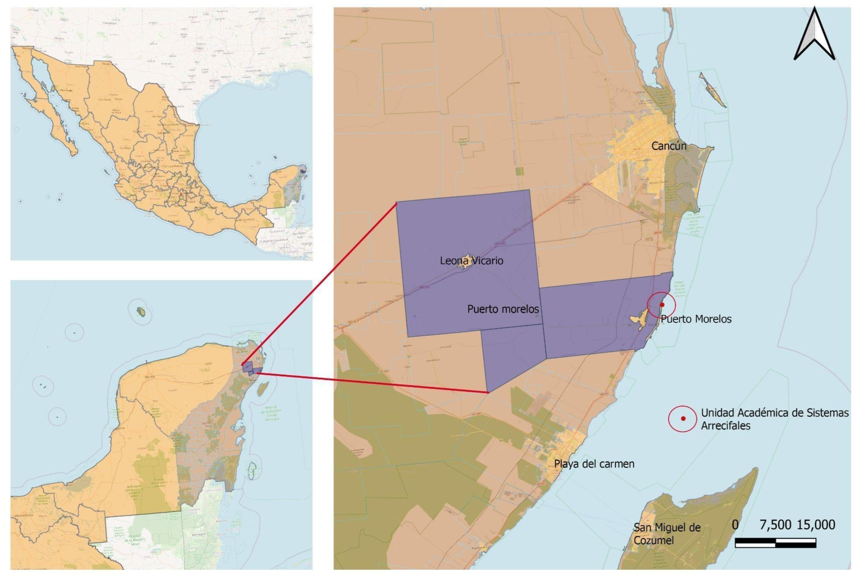
Figure 2.
Sample photography from EVMC.
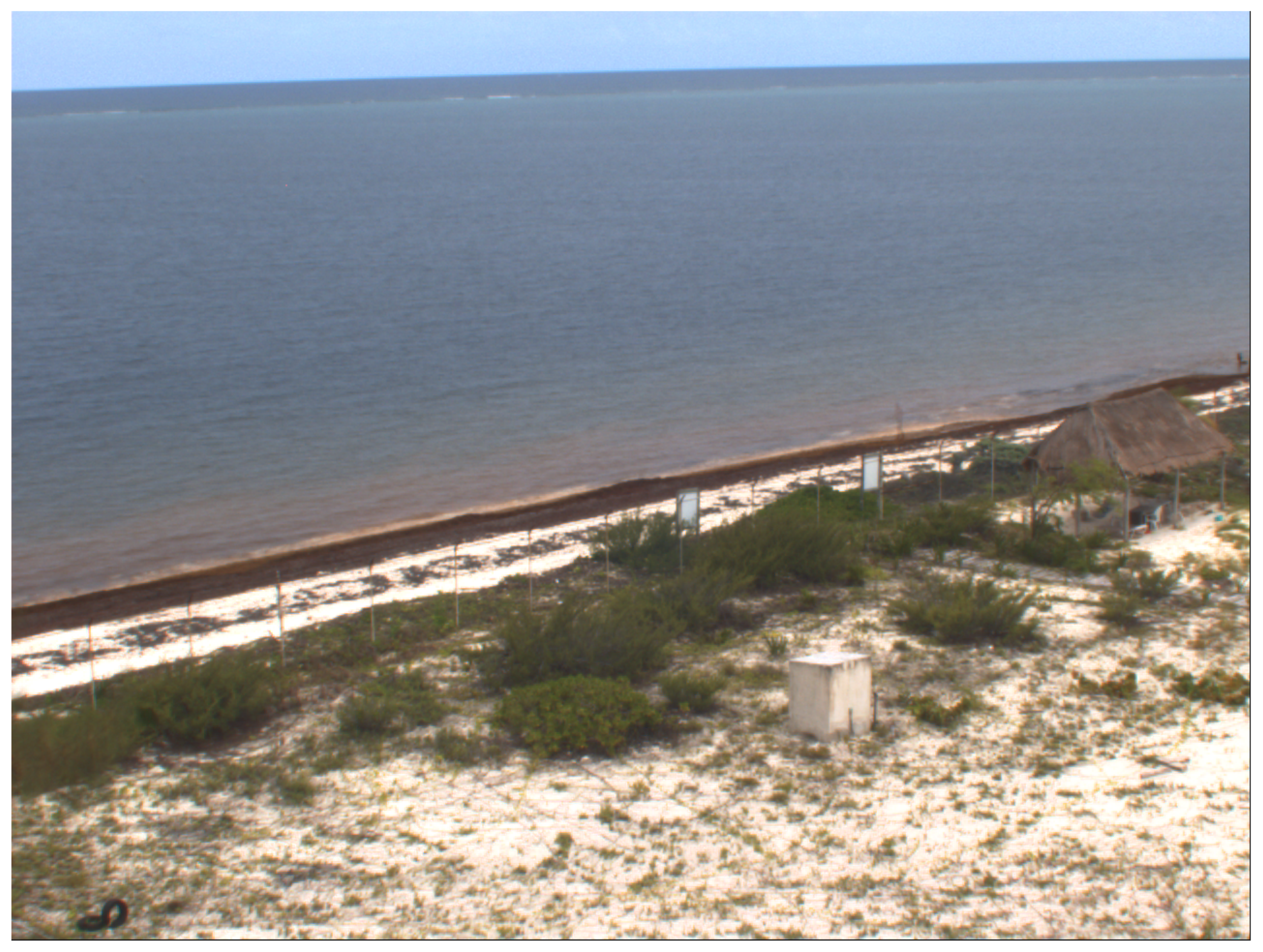
Figure 3.
Sample photography from Sentinel-2 with ROI for sargassum on a) sand b) water.
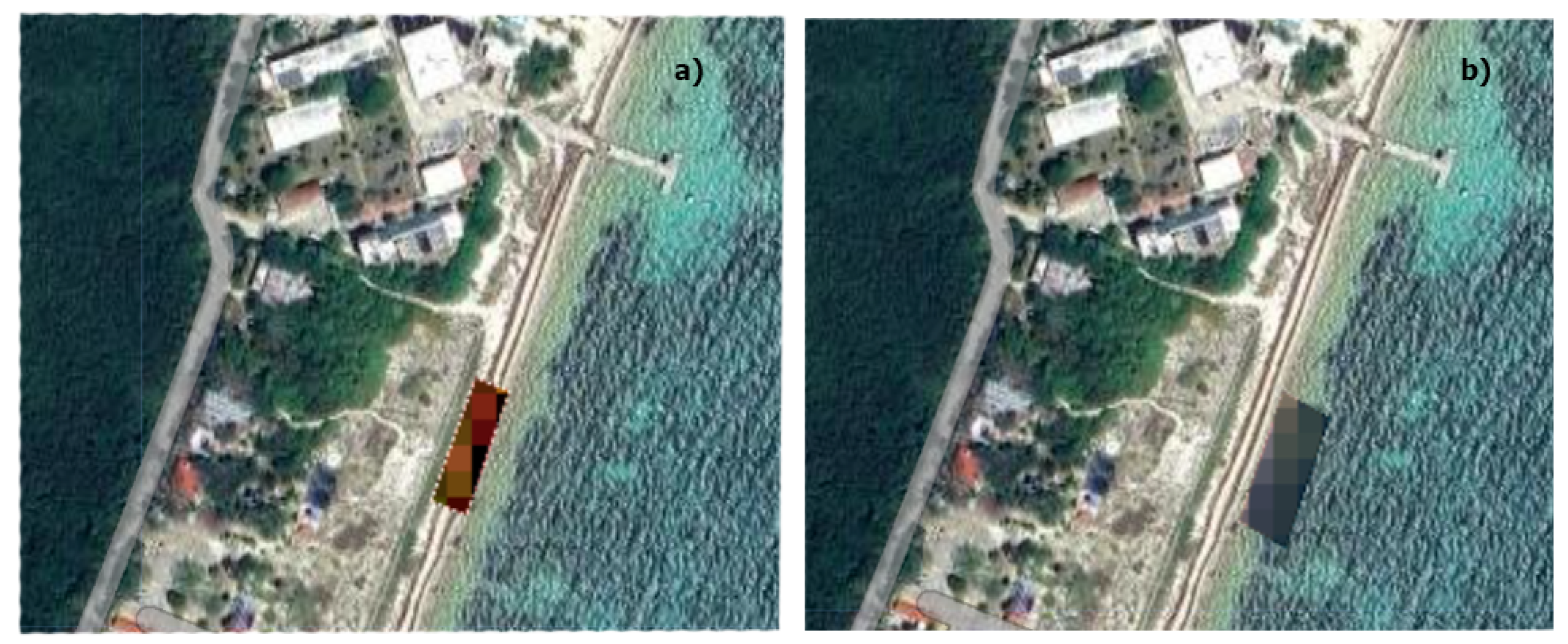
Figure 5.
Feature importance of the sargassum–sand model based on Gini impurity reduction.
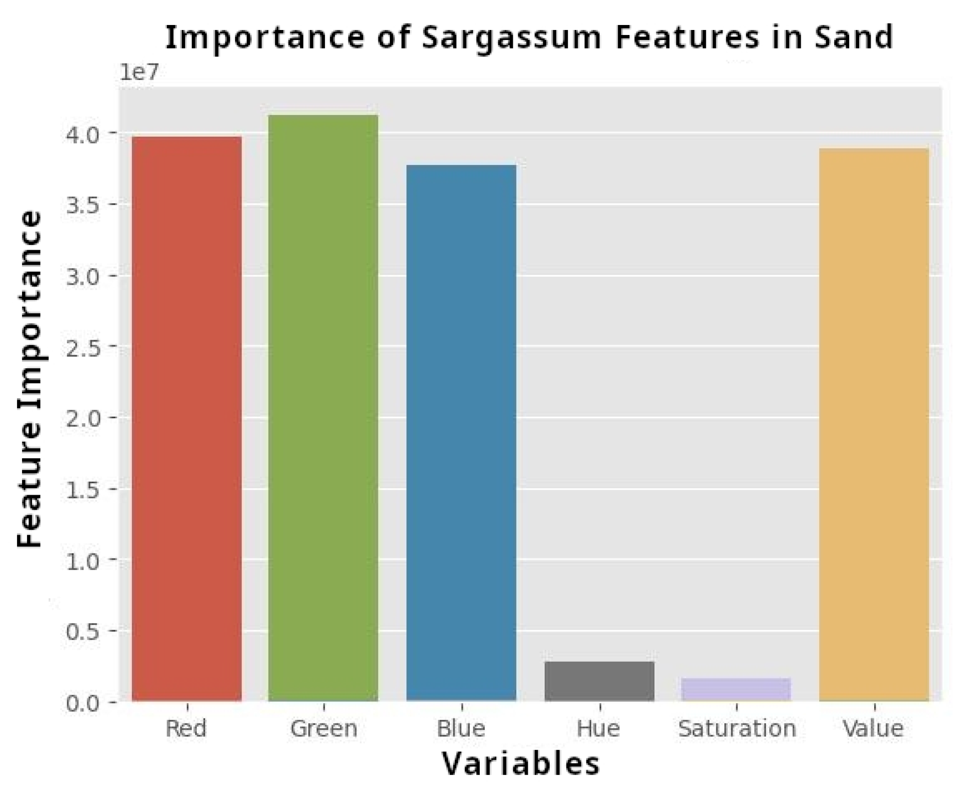
Figure 6.
Histograms illustrating the RGB distribution of the main elements in the image: sand, dry and wet Sargassum, vegetation, and water.
Figure 6.
Histograms illustrating the RGB distribution of the main elements in the image: sand, dry and wet Sargassum, vegetation, and water.
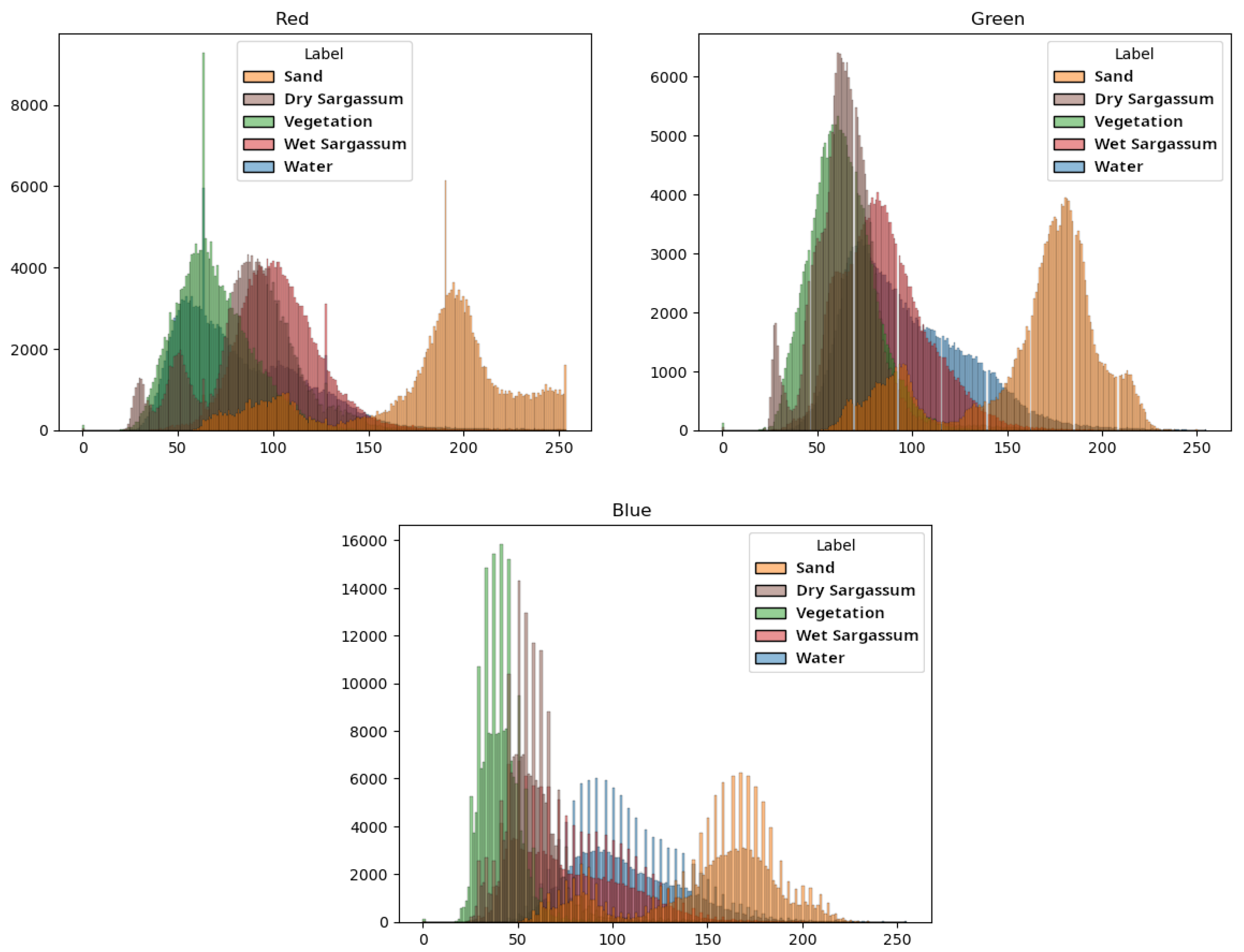
Figure 7.
Feature importance of the sargassum–water model based on Gini impurity reduction.
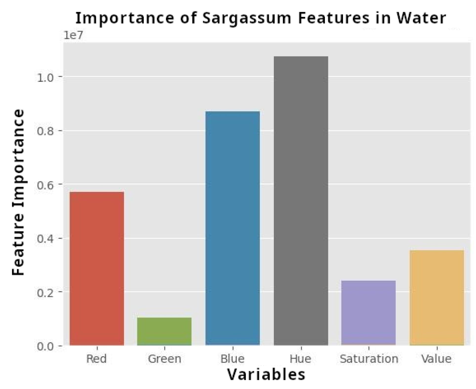
Figure 8.
Histograms illustrating the HSV distribution of the main elements in the image: sand, dry and wet sargassum, vegetation, and water.
Figure 8.
Histograms illustrating the HSV distribution of the main elements in the image: sand, dry and wet sargassum, vegetation, and water.
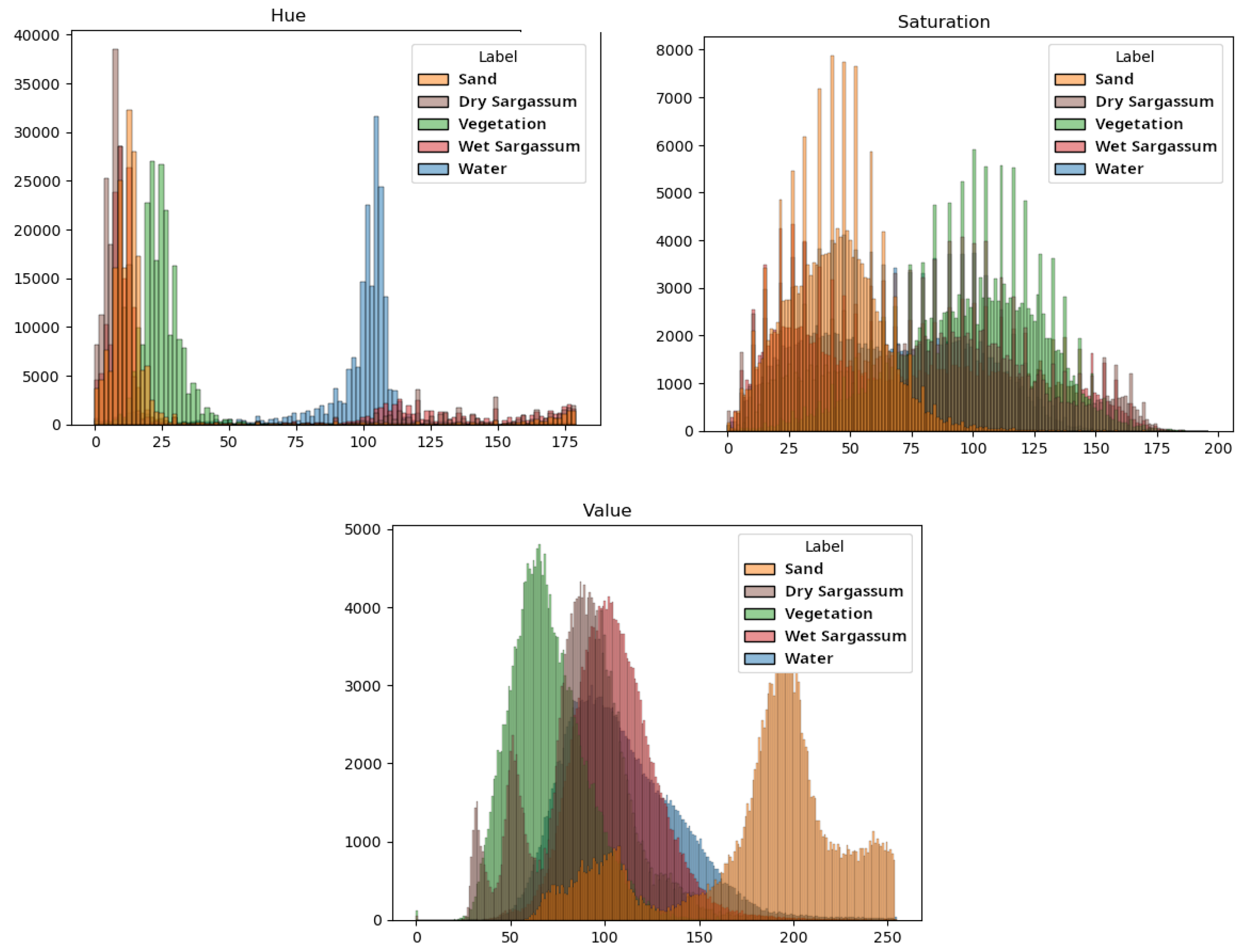
Figure 9.
Predictions of the different Machine Learning algorithms, the pixels detected as sargassum over the sand are colored in red.
Figure 9.
Predictions of the different Machine Learning algorithms, the pixels detected as sargassum over the sand are colored in red.
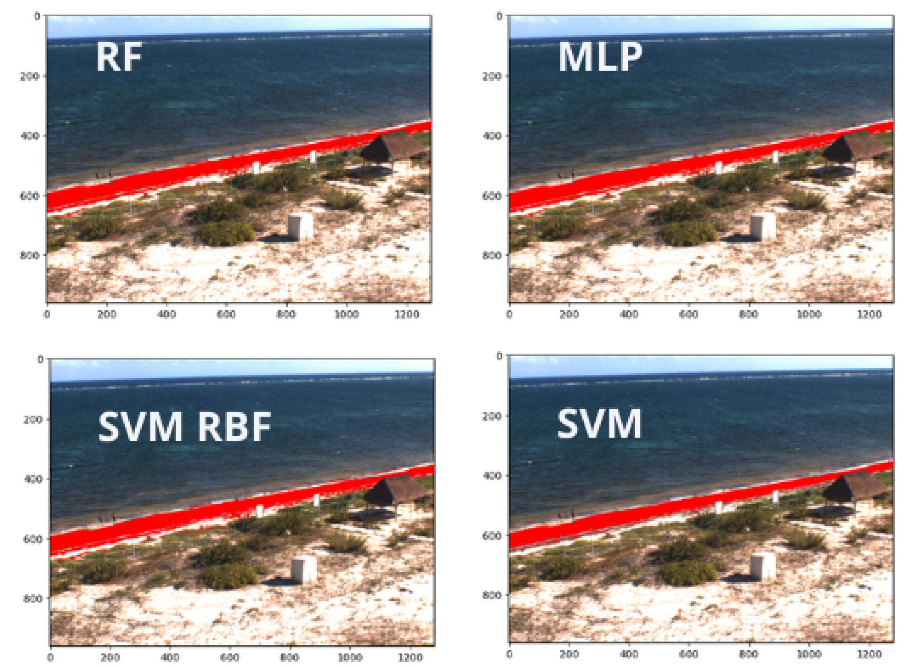
Figure 10.
Predictions of the different Machine Learning algorithms, the pixels detected as sargassum over the water are colored in red.
Figure 10.
Predictions of the different Machine Learning algorithms, the pixels detected as sargassum over the water are colored in red.
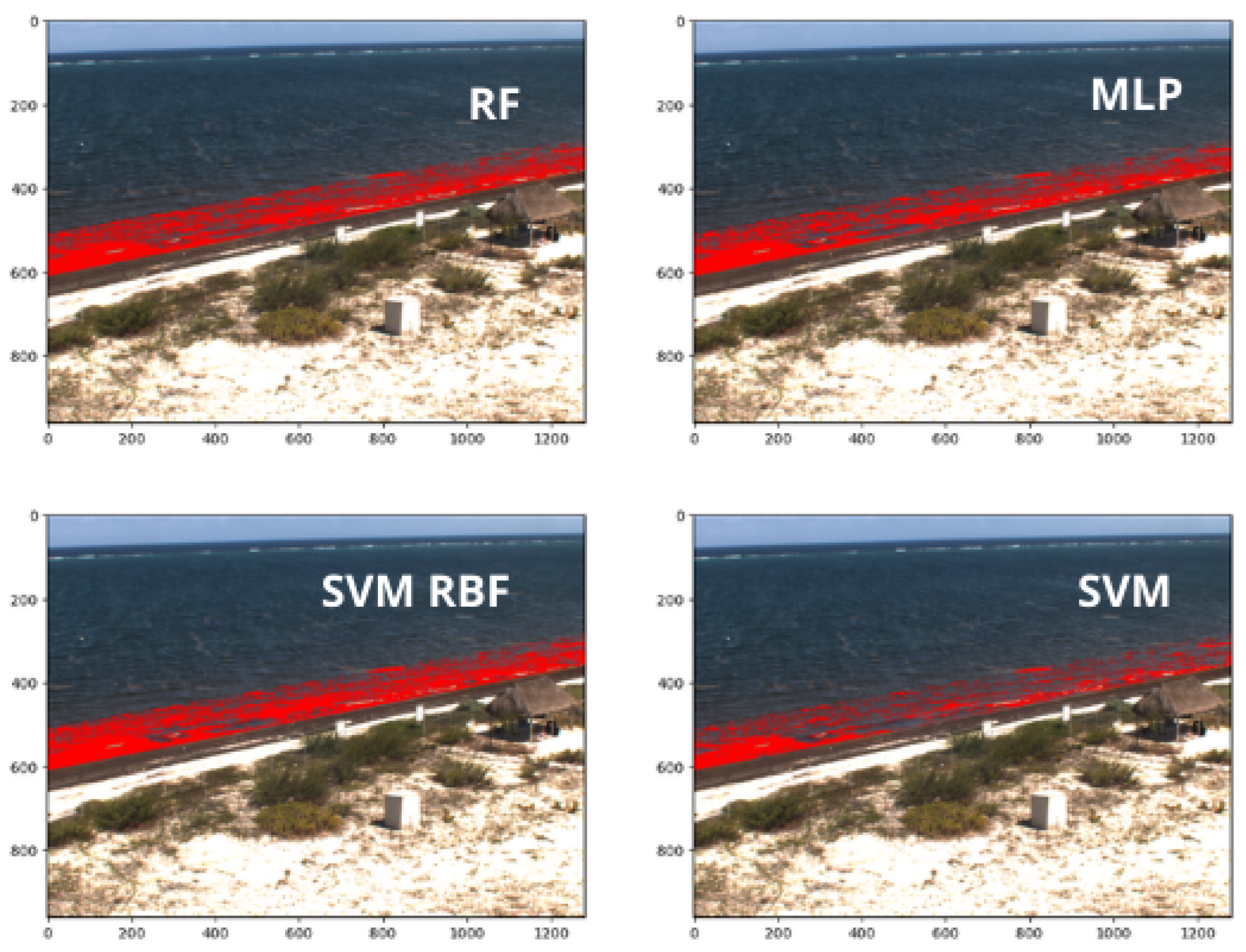
Figure 11.
Time series for the four ML models for sargassum prediction on sand.
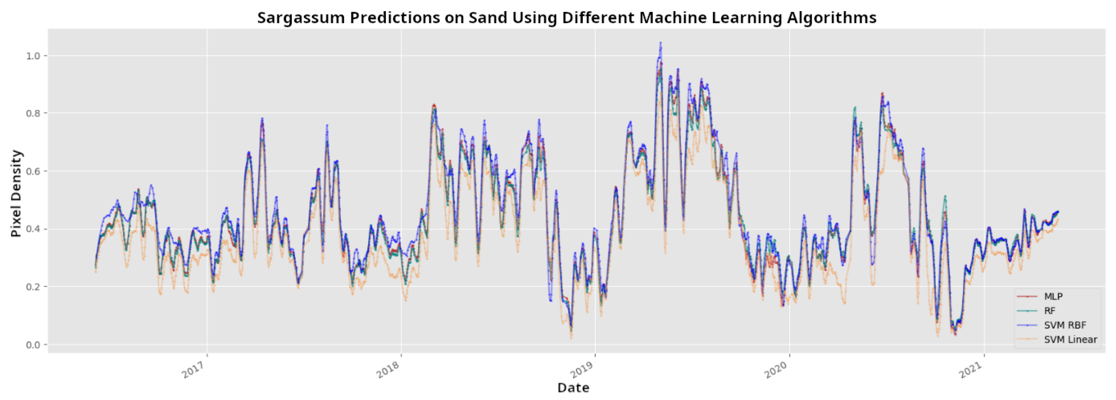
Figure 12.
Time series for the four ML models for sargassum prediction on water.
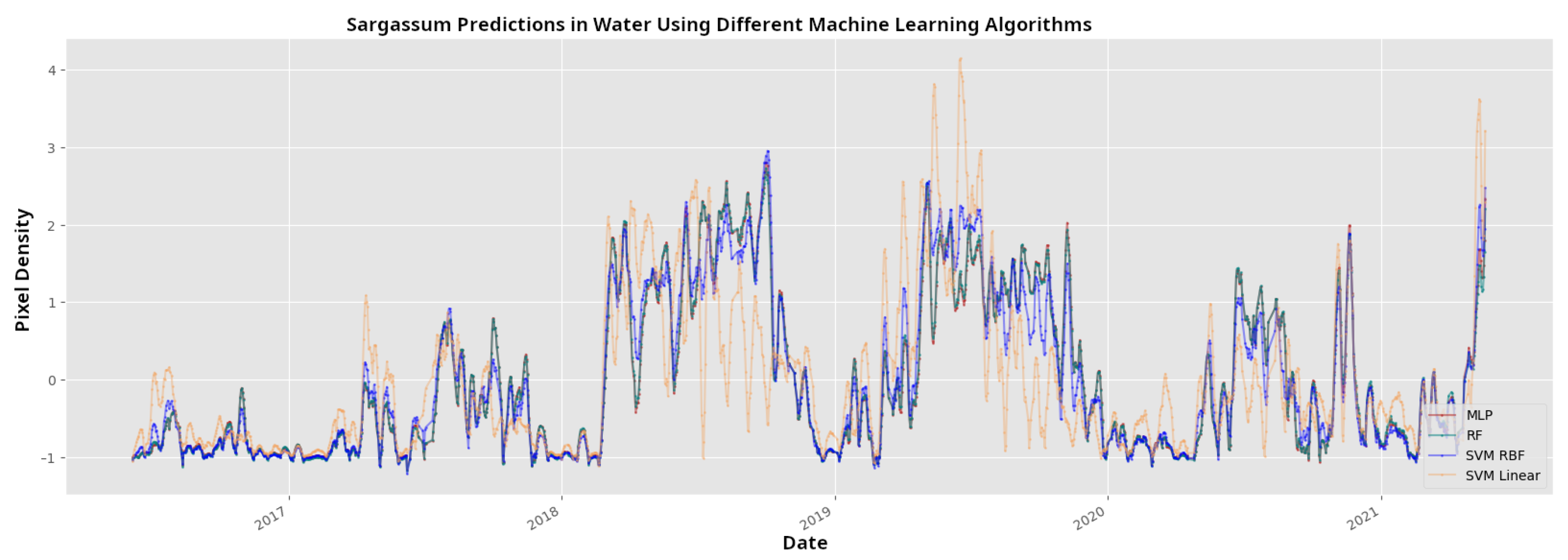
Table 1.
Performance metrics ML algorithms for sargassum detection on sand.
| Model | Metric | Test Set Score |
Cross Validation Average |
Training Time (s) |
Prediction Time (s) |
|---|---|---|---|---|---|
| Random Forest | F1-score | 0.8532 | 0.8532 | 218.029 | 5.8667 |
| Accuracy | 0.8570 | 0.8431 | |||
| Multilayer Perceptron | F1-score | 0.8898 | 0.8638 | 315.240 | 3.9469 |
| Accuracy | 0.8831 | 0.8614 | |||
| SVM RFB | F1-score | 0.8695 | 0.8586 | 244.302 | 870.755 |
| Accuracy | 0.8658 | 0.8531 | |||
| SVM Lineal | F1-score | 0.7905 | 0.7575 | 201.084 | 3.2037 |
| Accuracy | 0.8144 | 0.7571 |
Table 3.
Correlations coefficients between EVMC and satellite spectral indices.
| MLP (sand) Spearsman () |
RF (water) Pearson (r) |
|||
| Spectral Index | common dates | avg month | common dates | avg. month |
| NDVI | 0.614 | 0.635 | 0.734 | 0.753 |
| FAI | 0.392 | 0.405 | 0.689 | 0.736 |
Disclaimer/Publisher’s Note: The statements, opinions and data contained in all publications are solely those of the individual author(s) and contributor(s) and not of MDPI and/or the editor(s). MDPI and/or the editor(s) disclaim responsibility for any injury to people or property resulting from any ideas, methods, instructions or products referred to in the content. |
© 2025 by the authors. Licensee MDPI, Basel, Switzerland. This article is an open access article distributed under the terms and conditions of the Creative Commons Attribution (CC BY) license (https://creativecommons.org/licenses/by/4.0/).
Copyright: This open access article is published under a Creative Commons CC BY 4.0 license, which permit the free download, distribution, and reuse, provided that the author and preprint are cited in any reuse.


