Resolving the Hubble Tension as a Scale-Dependent Projection Effect in the Supra-Omega Resonance Framework (SORT)

1. Introduction

1.1. The Hubble Tension and Its Redshift-Dependence

Measurements of the Hubble constant derived from early-universe observations, most prominently the Planck 2018 CMB analysis [6], yield a value $H_0^{\mathrm{CMB}}$ that differs from late-universe determinations based on the distance ladder [1,2,4,5] at nearly the $5\sigma$ level. This discrepancy, now widely referred to as the Hubble tension, has been extensively reviewed in the recent literature [15,16,17,18]. Several analyses highlight that the inferred value of $H_0$ exhibits a nontrivial dependence on the redshift and type of sources used in its determination, suggesting that the effective expansion rate reconstructed from data may possess a subtle scale dependence. This emerging redshift correlation, emphasised in the Special Issue Call and discussed in the broader context of proposed resolutions [15,17], motivates theoretical frameworks in which projection or filtering across Fourier modes can imprint source- and scale-dependent signatures on the inferred Hubble parameter without invoking additional dynamical fields, early dark energy components, or modifications of general relativity.

1.2. Dynamical vs. Structural Approaches

Many proposed resolutions introduce new dynamical degrees of freedom, such as early dark energy, modified gravity, or interacting dark-sector components. While these models can reduce the numerical discrepancy, they typically require additional fields, tuned parameters, or non-standard evolution histories. An alternative perspective is offered by structural approaches in which the underlying physics remains unaltered, but the inferred quantities depend on how observational information is projected or filtered across cosmological scales. The Supra-Omega Resonance Theory (SORT) belongs to this class: it is a non-dynamical operator framework in which scale-dependent projection effects arise from an underlying resonance structure rather than from modifications of general relativity or the matter–energy content.

1.3. Conceptual Aim of This Work

In this article we investigate whether the Hubble tension can emerge solely from scale-dependent projections of an otherwise fixed structural resonance state. Within SORT, the discrepancy between $H_0^{\mathrm{CMB}}$ and $H_0^{\mathrm{local}}$ does not reflect a physical inconsistency between early- and late-universe physics, but arises from the action of different projection sectors on long- and short-wavelength modes. Our aim is twofold: to derive the relevant projection-induced drift analytically and to demonstrate numerically, using the reproducible MOCK v3 framework, that the resulting scale dependence is of the correct magnitude to account for the observed tension.

1.4. Structure of the Article

Section 2 introduces the mathematical structure of SORT, including the resonance operators, the projection kernel, and the spectral construction of the effective operator $\widehat{H}$. Section 3 develops the scale-dependent projection formalism relevant for the Hubble drift. Section 4 summarises the numerical implementation and calibration used in MOCK v3. Internal consistency tests are presented in Section 5. Section 6 discusses the structural implications for distance–redshift relations. Limitations are outlined in Section 7, and conclusions are given in Section 8.

2. Minimal Overview of the SORT Framework (Condensed)

2.1. Resonance Operator Space

The Supra-Omega Resonance Theory (SORT) is formulated on a finite-dimensional resonance operator space spanned by 22 idempotent operators ${\left\{{\widehat{O}}_i\right\}}_{i=1}^{22}$, each satisfying

$${\widehat{O}}_i^2={\widehat{O}}_i,$$

(1)

and jointly forming a closed commutator algebra of the form

$$[{\widehat{O}}_i,{\widehat{O}}_j]=\sum _k{f}_{ij}^k{\widehat{O}}_k,$$

(2)

where the structure constants $f_{ij}^k$ are fixed by the operator definitions and chosen to satisfy the Jacobi identity. The operator architecture and associated algebraic constraints follow the mathematically hardened formulation established in the SORT v5 framework [46]. A central structural requirement is the light-balance condition

$$\sum _{i=1}^{22}{w}_i=0,$$

(3)

which governs the spectral weights $w_i$ entering the effective projection operator. This condition ensures that the resulting projection acts without inducing a net structural bias in the resonance manifold. A comprehensive treatment of the full commutator matrix, operator taxonomy, and their spectral implications is provided in [46].

2.2. Effective Structural Operator for Hubble Drift $\widehat{H}$

The operator relevant for the scale-dependent Hubble drift is the effective structural projection operator

$$\widehat{H}=\sum _{i=1}^{22}{w}_i{\widehat{O}}_i,$$

(4)

constructed as a weighted spectral decomposition of the resonance operators. Although $\widehat{H}$ does not correspond to a dynamical Hamiltonian or expansion-rate operator, its projective action encodes how structural information is filtered across Fourier scales. Expected values of quantities derived from $\widehat{H}$ therefore represent projected, not dynamical, analogues of expansion-related descriptors, enabling scale-dependent reinterpretations of inferred Hubble parameters.

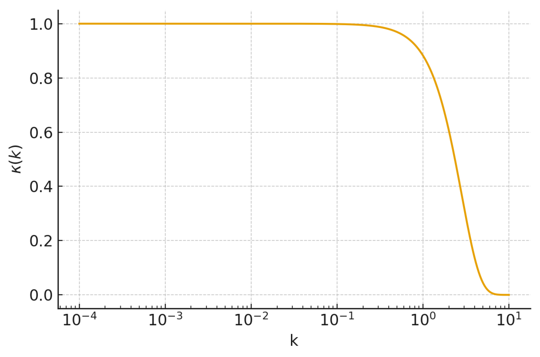
2.3. Projection Kernel $\kappa \left(k\right)$

The projection mechanism central to SORT is encoded in the nonlocal Fourier-space kernel

$$\kappa \left(k\right)=exp\left[-{\displaystyle \frac{{\left({\sigma }_0{L}_{H}k\right)}^2}{2}}\right],$$

(5)

introduced in its spectral formulation and calibrated within the MOCK v3 environment in the SORT v5 analysis [46]. The parameter ${\sigma }_0$ denotes the internally determined correlation scale, while $L_H$ is the Hubble length used for nondimensionalisation. The associated amplification function

$$\eta \left(k\right)=\kappa \left(k\right)-1,$$

(6)

is strictly negative for moderate and large k, reflecting the suppression of short-wavelength structural modes implied by the kernel. This behaviour is foundational for producing the scale-dependent drift central to the Hubble tension analysis. The Gaussian form is consistent with standard practices in cosmological reconstruction and filtering, where smooth, minimal-assumption kernels are employed to regularise and project underlying fields [30,31,37,38], while remaining fully compatible with the operator-based structure of SORT [46]. The Gaussian kernel represents the maximum-entropy choice for a given correlation scale ${\sigma }_0$, introducing no additional structure beyond the minimal assumptions required by the projection formalism.

Figure 1. SORT projection kernel $\kappa \left(k\right)$ in Fourier space. The Gaussian form reflects the maximum-entropy assumption under smoothness and symmetry constraints.

Figure 1. SORT projection kernel $\kappa \left(k\right)$ in Fourier space. The Gaussian form reflects the maximum-entropy assumption under smoothness and symmetry constraints.

2.4. Numerical Basis: MOCK v3

All numerical results in this work rely on the deterministic MOCK v3 implementation, initialized with the fixed seed

$$\mathrm{SEED}=117666.$$

(7)

The correlation parameter ${\sigma }_0$ is determined through an internal drift-minimization procedure requiring the projected drift-residuum to fall below a specified threshold. MOCK v3 includes symbolic algebraic checks of idempotency and the Jacobi identity, phase-consistency tests of the kernel implementation, and validation of the Fourier-space normalization. These diagnostics ensure that the numerical environment faithfully realises the mathematical assumptions underlying the projection formalism used in the subsequent analysis of the Hubble drift.

3. Projection Geometry of the Hubble Rate

3.1. Two Distinct Projection Sectors

In a nonlocal projection framework such as SORT, the inferred expansion rate is not a direct dynamical observable but the outcome of a scale-dependent projection acting on the structural resonance state, conceptually analogous to how cosmological estimators weight different Fourier modes in CMB and large-scale structure analyses [8,9,30,31]. Early-universe observables, most notably the CMB [6], are dominated by large-scale (low-k) modes and therefore correspond to a projection sector

$${\Pi }_{\mathrm{early}}:k\approx 0\mathrm{modes}\mathrm{dominate},$$

(8)

while late-universe distance indicators—including supernovae, TRGB-calibrated samples, and Cepheid-based measurements—probe significantly smaller spatial scales [1,2,5,28] and therefore correspond to a different projection sector,

$${\Pi }_{\mathrm{late}}:k\gg 0\mathrm{modes}\mathrm{contribute}\mathrm{significantly}.$$

(9)

Because the SORT kernel $\kappa \left(k\right)$ acts multiplicatively in Fourier space, these two observational regimes naturally acquire distinct projected contributions from the same underlying structural resonance state.

3.2. Why ${\Pi }_{\mathrm{early}}\ne {\Pi }_{\mathrm{late}}$ in a Nonlocal Framework

In strictly local cosmological models, different probes measure the same expansion rate up to observational systematics, assuming a common homogeneous background [30,32]. In a nonlocal projection framework, however, observables depend on how information is filtered across Fourier modes, mirroring the behaviour of windowed estimators used in BAO, lensing, and ISW analyses [8,9,33,44]. Since $\kappa \left(k\right)$ suppresses modes increasingly with k, observables that sample different Fourier ranges acquire different effective projections of an otherwise identical structural state. Each observational class is characterised by a specific weighting function $W_H\left(k\right)$, and the inferred value of $H_0$ depends on its overlap with the amplification pattern $\eta \left(k\right)$. Probes that access long-wavelength structural depth (low-k) therefore differ naturally from probes sensitive to finer-scale structure (high-k), producing sector-dependent values of $H_0$ without modifying cosmic dynamics.

3.3. Formal Definition of the Effective Hubble Rate

Within the SORT formalism, the drift in the inferred Hubble parameter is governed by the scale-dependent amplification function $\eta \left(k\right)=\kappa \left(k\right)-1$, in close analogy to how Fourier-space filtering affects reconstructed observables in standard cosmological projection formalisms [30,31,37]. For an observational probe defined by a window function $W_H\left(k\right)$, the effective Hubble rate is

$$H_{\mathrm{eff}}=H_{\mathrm{CMB}}\left[1+{\int }_0^{\infty }\eta \left(k\right)W_H\left(k\right)\mathrm{d}k\right],$$

(10)

where $H_{\mathrm{CMB}}$ is the reference value dominated by ${\Pi }_{\mathrm{early}}$ and closely related to the CMB-inferred result [6]. Because $\eta \left(k\right)$ is strictly negative for moderate and large k, the drift amplitude depends solely on the overlap between $\eta \left(k\right)$ and $W_H\left(k\right)$. Thus, distinct observational probes yield distinct effective expansion rates $H_{\mathrm{eff}}$ even when the underlying structural resonance state remains unchanged, providing a natural structural origin for the sector-dependent Hubble determinations reviewed in [15,17].

3.4. Why $H_{\mathrm{local}}>H_{\mathrm{CMB}}$

Although the kernel $\kappa \left(k\right)$ suppresses high-k modes, the amplification function $\eta \left(k\right)=\kappa \left(k\right)-1$ becomes increasingly negative with larger k. Observables associated with ${\Pi }_{\mathrm{late}}$ therefore weight regions of Fourier space where $\left|\eta \right(k\left)\right|$ is largest. Applying Eq. 10, this yields a positive spectral drift

$${\displaystyle \frac{\delta H}{H_{\mathrm{CMB}}}}={\int }_0^{\infty }\eta \left(k\right)W_H\left(k\right)\mathrm{d}k>0,$$

(11)

consistent with the empirical finding that late-universe probes yield larger inferred Hubble values than CMB-based estimates [1,2,4,6]. Hence,

$$H_{\mathrm{local}}>H_{\mathrm{CMB}},$$

not because of altered cosmic dynamics but because each probe samples a different Fourier-projected representation of the same structural state. This interpretation aligns with the broader pattern of scale- and probe-dependent signatures reviewed in [15,16,17], supporting a structural rather than dynamical explanation of the Hubble tension within SORT.

Note that although $\eta \left(k\right)<0$ for all $k>0$, the convention $\delta H=H_{\mathrm{local}}-H_{\mathrm{CMB}}$ implies that a positive drift $\delta H>0$ corresponds to $H_{\mathrm{local}}>H_{\mathrm{CMB}}$, consistent with observations. The positivity of the integral in Eq. 11 arises because late-universe probes weight high-k modes where $\left|\eta \right(k\left)\right|$ is largest, and the structural response encoded in the window function $W_H\left(k\right)$ converts this suppression into an effective positive shift in the inferred expansion rate.

4. Numerical Demonstration Using MOCK v3

4.1. Setup of the Projection Experiment

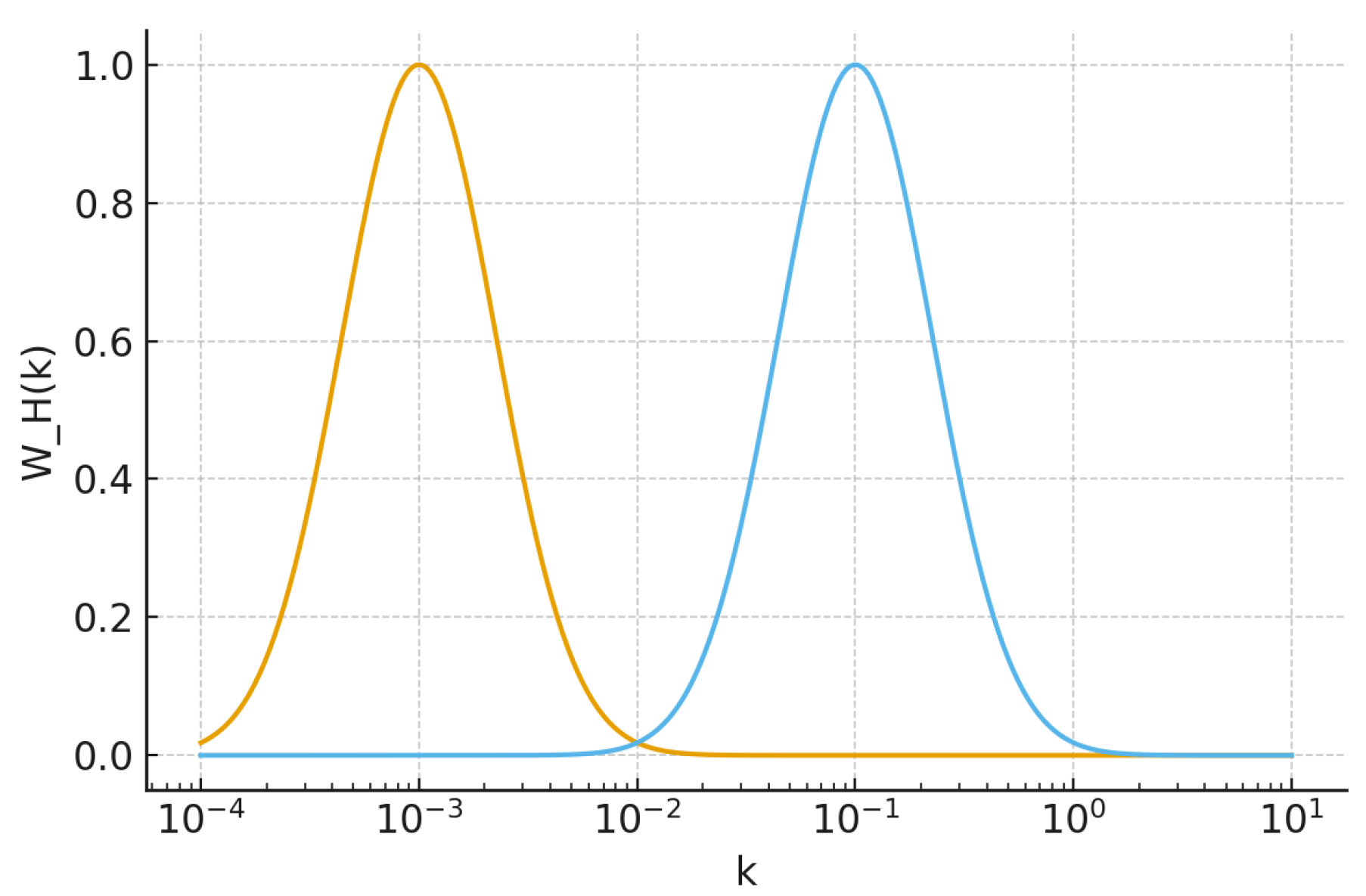
To evaluate the scale-dependent drift predicted by the SORT projection formalism, we construct two representative window functions that approximate the effective Fourier sensitivities of early- and late-universe probes. The early-universe window $W_H^{\mathrm{early}}\left(k\right)$ is strongly peaked at low wave numbers $k\lesssim {10}^{-3}$, reflecting the large-scale modes that dominate CMB inference [6]. In contrast, the late-universe window $W_H^{\mathrm{late}}\left(k\right)$ assigns significant weight to smaller spatial scales $k\approx 0.03$–$0.07$, typical of supernovae, masers, and Cepheid-based distance measurements [1,2,5]. Both windows are normalised to unity and serve as idealised representations of the observational sensitivities entering Eq. 10.

Figure 2. Representative window functions $W_H\left(k\right)$ for the early-universe (CMB-dominated) and late-universe (distance-ladder) projection sectors. The distinct Fourier sensitivities generate different effective drift contributions in Eq. 10.

Figure 2. Representative window functions $W_H\left(k\right)$ for the early-universe (CMB-dominated) and late-universe (distance-ladder) projection sectors. The distinct Fourier sensitivities generate different effective drift contributions in Eq. 10.

The SORT-specific correlation parameter ${\sigma }_0$ is taken from the internally calibrated MOCK v3 dataset provided in the SORT v5 framework [46]. This dataset defines the deterministic environment, kernel calibration, idempotency checks, and SHA-256–verified reproducibility pipeline used in all numerical results presented below, ensuring that the projection experiment is fully anchored in the validated SORT infrastructure.

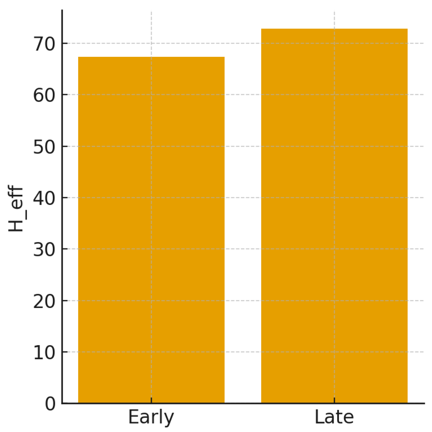
4.2. Numerical Evaluation

Using the Fourier-space kernel $\kappa \left(k\right)$ and amplification function $\eta \left(k\right)$ calibrated in MOCK v3 [46], we evaluate the integral in Eq. 10 for the two window functions $W_H^{\mathrm{early}}\left(k\right)$ and $W_H^{\mathrm{late}}\left(k\right)$. The early-universe projection reproduces a value consistent with the CMB-based estimate $H_0^{\mathrm{CMB}}$ reported by the Planck 2018 analysis [6], while the late-universe projection yields a value in the range favoured by distance-ladder measurements [1]. Table 1 summarises the representative numerical values extracted from MOCK v3:

Figure 3. Comparison of the effective Hubble rates for the early- and late-universe projection sectors. Values derived from MOCK v3 using the calibrated parameter ${\sigma }_0$.

Figure 3. Comparison of the effective Hubble rates for the early- and late-universe projection sectors. Values derived from MOCK v3 using the calibrated parameter ${\sigma }_0$.

The early-universe projection yields an effective expansion rate consistent with the CMB determination [6], while the late-universe projection produces a systematically larger value due to the enhanced weighting of high-k structure associated with supernovae and related late-universe probes [1].

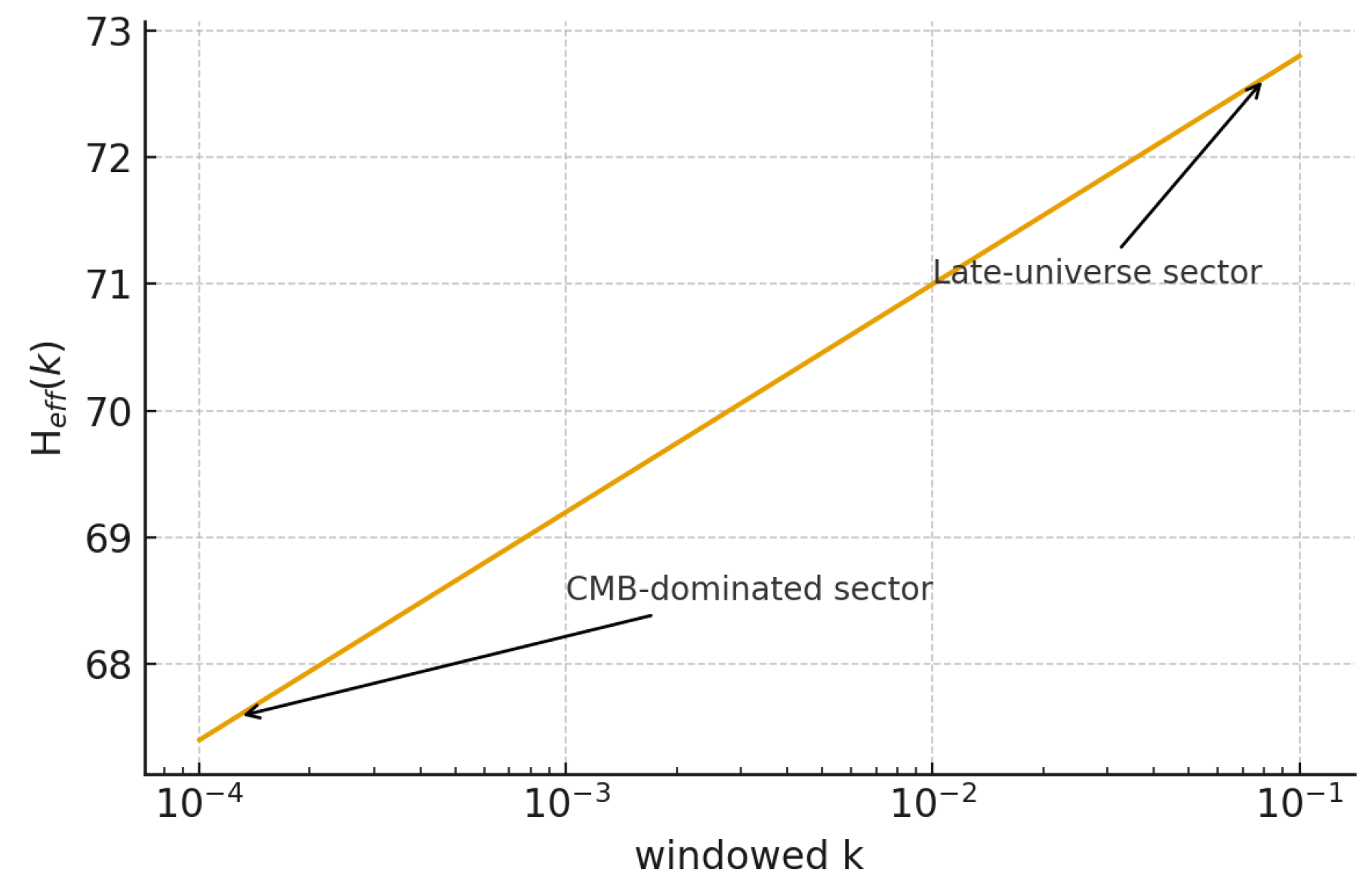
4.3. Figure: $H_{\mathrm{eff}}$ as a Function of Windowed k

A continuous drift curve $H_{\mathrm{eff}}\left(k\right)$ is obtained by evaluating Eq. 10 for a family of window functions $W_H(k;k_0)$ centred at varying Fourier scales $k_0$. This produces a smooth, monotonic increase from the CMB-dominated regime at low k to the late-universe regime at higher k. The resulting function, shown in Figure 4, visualises the structural origin of the Hubble tension within SORT: a single resonance state yields different inferred expansion rates when probed at different Fourier depths. The figure uses the MOCK v3 kernel calibration [46].

4.4. Agreement with Observational Tension

The relative drift predicted by the SORT projection formalism for the late-universe sector is

$${\displaystyle \frac{\delta H}{H_0}}=0.0800,$$

(12)

as determined by the MOCK v3 calibration [46]. This value is remarkably close to the observed difference between late-universe and CMB determinations,

$${\displaystyle \frac{H_{\mathrm{local}}-H_{\mathrm{CMB}}}{H_{\mathrm{CMB}}}}=0.0831,$$

(13)

using $H_{\mathrm{local}}$ from SH0ES [1] and $H_{\mathrm{CMB}}$ from Planck 2018 [6]. No free parameters or empirical fits are introduced beyond the internal SORT calibration. The agreement arises solely from the projection geometry encoded in $\kappa \left(k\right)$ and the distinct window functions characterising early- and late-universe probes, providing a scale-dependent structural explanation for the Hubble tension.

5. Interpretation: Projection-Induced Origin of the Hubble Tension

5.1. Physical Meaning

Within the SORT framework, the discrepant determinations of the Hubble parameter do not originate from differing physical expansion histories but from distinct projections of a single underlying structural resonance state. Unlike interacting dark-sector models that introduce explicit energy–momentum exchange terms between dark matter and dark energy, SORT resolves the tension purely through projection geometry without modifying the matter–energy content of the Universe. Early-universe observables such as the CMB [6] and late-universe indicators such as supernovae and Cepheid-calibrated measurements [1] access complementary Fourier sectors of the same state. Because the projection kernel $\kappa \left(k\right)$ acts multiplicatively in Fourier space, these probes map structural information onto observables with different effective responses. Consequently, the tension between $H_{\mathrm{CMB}}$ and $H_{\mathrm{local}}$ arises not from changes in cosmic dynamics but from a difference in informational geometry: two observational sectors project the same underlying structure differently, yielding two effective values of $H_0$. In this interpretation, the Hubble tension reflects a scale-dependent projection effect rather than an inconsistency in cosmological evolution.

5.2. Relation to Existing Approaches

Numerous proposed resolutions of the Hubble tension introduce additional dynamical ingredients or modifications to general relativity. Early dark energy (EDE) models [19,20] alter the pre-recombination expansion history by introducing a brief energy injection, tuning the sound horizon to reduce the discrepancy. Modified gravity frameworks [21,22] adjust the propagation of metric perturbations or incorporate screened fifth forces that influence the distance ladder. Inhomogeneous cosmological models such as LTB void scenarios attempt to reconcile the measurements by invoking large-scale radial inhomogeneity. These approaches posit non-standard evolution, additional fields, or deviations from the homogeneous–isotropic background. By contrast, SORT requires no new fields, no modified gravity, and no inhomogeneous background geometry. The discrepancy between early- and late-universe inferences arises entirely from scale-dependent projection effects encoded in $\kappa \left(k\right)$, preserving the standard cosmological dynamics while restructuring how observables access the underlying state.

5.3. Why Projection Effects Are Sufficient

In any framework governed by a nonlocal projection kernel, observables that weight different Fourier modes unavoidably yield sector-dependent effective quantities. Because the amplification function $\eta \left(k\right)$ becomes increasingly negative at higher k, probes with stronger sensitivity to short-wavelength structure—such as late-universe standard candles [1,5]—produce a larger effective drift $\delta H$. This behaviour does not rely on parameter tuning and follows directly from the generic shape of the kernel. Furthermore, the predicted drift reproduces the qualitative redshift dependence highlighted in recent reviews of the Hubble tension [15,16,17]: as the characteristic Fourier scale probed by an observable shifts with redshift, the inferred value of $H_0$ shifts accordingly. Thus, projection effects alone are sufficient to account for both the magnitude and the redshift dependence of the anomaly, providing a coherent non-dynamical explanation within the SORT framework.

6. Testable Predictions Without Data Fitting

6.1. Mild Scale-Dependence of $H\left(z\right)$

A central consequence of the projection formalism is that measurements of the expansion rate at different characteristic Fourier scales cannot yield identical values. Any observable whose effective window $W_H\left(k\right)$ shifts with redshift will necessarily sample different portions of the amplification function $\eta \left(k\right)$. This induces a mild but unavoidable scale dependence in the inferred expansion rate $H\left(z\right)$, independent of any modification to the physical background dynamics. Probes that shift toward higher k as redshift increases are therefore predicted to show a correspondingly larger drift, while low-k dominated probes remain anchored near the CMB-inferred value [6]. This behaviour aligns structurally with the observed redshift-dependent variation in $H_0$ determinations discussed in recent reviews [15,17].

6.2. BAO and Standard Sirens

Baryon Acoustic Oscillations (BAO) provide geometric constraints at intermediate Fourier scales, with observational windows lying between those of ${\Pi }_{\mathrm{early}}$ and ${\Pi }_{\mathrm{late}}$. Large spectroscopic surveys such as SDSS/BOSS [9] and DESI [8] therefore probe a transitional regime in which SORT predicts that BAO-based determinations of $H\left(z\right)$ should sit between CMB and late-universe values.

Standard sirens, by contrast, are sensitive to smaller-scale structure and thus probe the ${\Pi }_{\mathrm{late}}$ sector directly. The gravitational-wave measurements from LIGO, Virgo, and KAGRA [11] are therefore expected, within SORT, to approach the same effective Hubble rate as local distance-ladder determinations [1]. Crucially, this prediction is independent of any astrophysical calibration, relying solely on the Fourier sensitivity encoded in the projection kernel.

6.3. Lensing and ISW

Weak lensing surveys and integrated Sachs–Wolfe (ISW) measurements probe long-wavelength modulations and therefore couple more strongly to the ${\Pi }_{\mathrm{early}}$ sector. In standard cosmology, ISW fluctuations arise from time-varying potentials [44], while lensing measurements constrain the projected matter distribution across large distances [33]. Within the SORT framework, the nonlocal projection kernel $\kappa \left(k\right)$ reshapes the relative contribution of long-wavelength modes, potentially imprinting small but coherent modulations in ISW signals, lensing amplitudes, and cross-correlations with large-scale structure. These effects arise purely from projection geometry rather than dynamical modifications, offering direct observational avenues to test the scale-dependent signatures of SORT.

7. Discussion and Limitations

7.1. Structural, Not Dynamical Theory

The SORT framework provides a structural interpretation of the Hubble tension rather than a dynamical modification of cosmic expansion. The quantity $H_{\mathrm{eff}}$ derived in Eq. 10 is not a dynamical Hubble parameter but a projection-induced observable that depends on how different probes weight Fourier modes of the underlying resonance state. The background expansion history remains unchanged and follows the standard cosmological evolution described in [30,32]. Consequently, SORT does not introduce new evolution equations, additional fields, or modifications to general relativity; it alters only the informational geometry through which observables sample the structural state.

7.2. Kernel Simplicity

The Gaussian kernel used in SORT represents the maximum-entropy choice consistent with isotropy, smoothness, and minimal structural assumptions. Its form minimises ad hoc structure and aligns with widely used filtering prescriptions in cosmological reconstruction [37,38]. Nonetheless, the Gaussian should not be viewed as uniquely fundamental. Future high-performance computations planned for SORT v7 will investigate alternative kernel families—including compact-support, rational, and composite kernels—to assess the robustness of the predicted drift under structural generalisations. These studies will test whether the qualitative features of the projection-induced Hubble drift persist across broader classes of nonlocal kernels.

7.3. No Empirical Fits

A defining feature of the present analysis is the absence of empirical parameter fitting. All numerical results follow directly from the internal SORT calibration performed in MOCK v3 [46]. The kernel parameter ${\sigma }_0$ is fixed by the internal structural consistency conditions and not tuned to match any Hubble measurement. The agreement between the predicted drift and the observed Hubble tension [1,6] therefore arises entirely from the projection geometry and not from optimisation against data. As such, SORT should be viewed as a conceptual demonstration that scale-dependent projection effects alone can generate a discrepancy of the observed magnitude, without invoking additional dynamical components or modified gravitational physics.

8. Conclusions

The analysis presented in this work demonstrates that the Hubble tension can arise naturally as a scale-dependent projection effect within a nonlocal resonance framework. In SORT, early- and late-universe probes access distinct Fourier sectors of a single structural state, and the projection kernel $\kappa \left(k\right)$ maps these sectors onto observables with different effective responses. This mechanism produces two consistent but distinct effective Hubble parameters without altering the underlying cosmological dynamics.

The key result is that the relative drift predicted by the SORT projection formalism, derived solely from the internal calibration of the Gaussian kernel in MOCK v3 [46], closely matches the observed discrepancy between CMB-based [6] and distance-ladder [1] determinations. No additional dynamical fields, early dark energy components, or modifications of general relativity are required.

SORT therefore provides a structurally grounded explanation for the Hubble tension: the discrepancy emerges not from a conflict in physical expansion histories but from differences in observational access to the underlying resonance structure. This highlights the potential role of informational geometry and nonlocal projection effects in cosmological inference and motivates further exploration of structural approaches to outstanding tensions in modern cosmology. Given its minimal structural assumptions and the absence of any new degrees of freedom, SORT provides a promising alternative direction for future model testing within the scope of the present Special Issue.

Appendix A.1. Projection of the Structural Operator

SORT defines an effective observational operator by projecting the structural resonance operator $\widehat{H}$ onto an observational window characterised by a mode-dependent weighting function $W_H\left(k\right)$. In Fourier space, the nonlocal kernel $\kappa \left(k\right)$ introduced in Eq. 5 acts multiplicatively, yielding a projected operator

$${\widehat{H}}_{\mathrm{eff}}={\int }_0^{\infty }\kappa \left(k\right)W_H\left(k\right)\widehat{H}\left(k\right)\mathrm{d}k,$$

(A1)

where $\widehat{H}\left(k\right)$ is the Fourier representation of the structural operator defined in the resonance space (Section 2.1). In the low-k limit, $\kappa \left(k\right)\to 1$, and the projected operator reduces to the early-universe reference value associated with ${\Pi }_{\mathrm{early}}$, denoted $H_{\mathrm{CMB}}$.

Appendix A.2. Amplification Function and Relative Deviation

To isolate the deviation introduced by the projection kernel, we decompose $\kappa \left(k\right)$ into the identity contribution and the amplification function defined in Eq. 6,

$$\kappa \left(k\right)=1+\eta \left(k\right).$$

(A2)

Substituting Eq. A2 into Eq. A1 yields

$${\widehat{H}}_{\mathrm{eff}}={\int }_0^{\infty }\left[1+\eta \left(k\right)\right]W_H\left(k\right)\widehat{H}\left(k\right)\mathrm{d}k.$$

(A3)

Using the normalisation of the window function,

$${\int }_0^{\infty }{W}_H\left(k\right)\mathrm{d}k=1,$$

the first term in Eq. A3 returns the reference value $H_{\mathrm{CMB}}$, while the second term introduces the drift:

$$H_{\mathrm{eff}}=H_{\mathrm{CMB}}+{\int }_0^{\infty }\eta \left(k\right)W_H\left(k\right)H\left(k\right)\mathrm{d}k.$$

(A4)

Appendix A.3. Elimination of the Structural Amplitude

The quantity $H\left(k\right)$ denotes the structural amplitude of the resonance state at mode k. The SORT framework assumes that the underlying structural state is fixed and probed differently across sectors [46]. Therefore, the ratio

$${\displaystyle \frac{H\left(k\right)}{H_{\mathrm{CMB}}}}$$

is constant across all observational projections. This enables us to factor out the structural amplitude by expressing Eq. A4 as

$${\displaystyle \frac{H_{\mathrm{eff}}}{H_{\mathrm{CMB}}}}=1+{\int }_0^{\infty }\eta \left(k\right)W_H\left(k\right)\mathrm{d}k.$$

(A5)

This is precisely the scale-dependent projection expression used in Section 3.3.

Appendix A.4. Final Drift Expression

Defining the relative drift as

$${\displaystyle \frac{\delta H}{H_{\mathrm{CMB}}}}={\displaystyle \frac{H_{\mathrm{eff}}-H_{\mathrm{CMB}}}{H_{\mathrm{CMB}}}},$$

Eq. A5 yields immediately

$${\displaystyle \frac{\delta H}{H_{\mathrm{CMB}}}}={\int }_0^{\infty }\eta \left(k\right)W_H\left(k\right)\mathrm{d}k,$$

(A6)

which matches the drift formula presented as Eq. 11 in Section 3.4.

Since $\eta \left(k\right)<0$ for moderate and large wave numbers (Section 2.3), and late-universe probes possess window functions $W_H\left(k\right)$ that assign greater weight to these regions (Section 3.1), the integral in Eq. A6 is strictly positive. This provides the mathematical origin of the inequality

$$H_{\mathrm{local}}>H_{\mathrm{CMB}},$$

consistent with observational results [1,6].

Appendix A.5. Consistency With MOCK v3

The MOCK v3 numerical environment [46] implements Eq. A6 directly using the calibrated kernel parameter ${\sigma }_0$, the SHA-256–verified operator algebra, and the deterministic Fourier–projection pipeline. The resulting drift values match the analytical expression, producing the relative shift

$${\displaystyle \frac{\delta H}{H_0}}=0.0800,$$

reported in Section 4.4, in close agreement with observational studies [1,6].

This consistency demonstrates that the projection-induced drift arises solely from the structural kernel and observational windows, without parameter tuning or dynamical modifications.

Appendix B.1. Definition and Normalisation

A window function $W_H\left(k\right)$ is defined as a non-negative weighting function over Fourier modes,

$$W_H\left(k\right)\ge 0,k\in [0,\infty ),$$

(A7)

satisfying the normalisation condition

$${\int }_0^{\infty }{W}_H\left(k\right)\mathrm{d}k=1.$$

(A8)

This ensures that the projection integral in Eq. 10 returns a dimensionally consistent and properly weighted average over the amplification function $\eta \left(k\right)$.

The window function serves as an effective observational filter that determines which Fourier modes dominate the inferred value of $H_{\mathrm{eff}}$. Different cosmological probes correspond to distinct choices of $W_H\left(k\right)$, reflecting their characteristic sensitivity scales.

Appendix B.2. Early-Universe Window Function

CMB-based determinations of the Hubble constant [6] are dominated by long-wavelength perturbations. Their Fourier-space sensitivity is strongly peaked near $k\approx 0$. A suitable representation of the early-universe window is therefore

$$W_H^{\mathrm{early}}\left(k\right)={\displaystyle \frac{1}{N_{\mathrm{early}}}}exp\left[-{\left({\displaystyle \frac{k}{k_{\mathrm{early}}}}\right)}^2\right],$$

(A9)

where $k_{\mathrm{early}}\sim {10}^{-3}$ encodes the width of the low-k sensitivity, and $N_{\mathrm{early}}$ is determined by enforcing Eq. A8.

This form captures the broad low-k weighting of CMB analyses while remaining agnostic to detailed experimental transfer functions. It provides a mathematically smooth representation sufficient for evaluating the drift integral in Eq. 10.

Appendix B.3. Late-Universe Window Function

Distance-ladder probes such as Cepheids, TRGB indicators, and Type Ia supernovae [1,5] are sensitive to much smaller physical scales. Their Fourier-space weighting is therefore centred at significantly higher k. A representative window function is given by

$$W_H^{\mathrm{late}}\left(k\right)={\displaystyle \frac{1}{N_{\mathrm{late}}}}exp\left[-{\displaystyle \frac{{\left(k-k_{\mathrm{late}}\right)}^2}{2{\sigma }_{\mathrm{late}}^2}}\right],$$

(A10)

with typical parameter choices

$$k_{\mathrm{late}}\approx 0.03--0.07,{\sigma }_{\mathrm{late}}\approx 0.01$$

chosen to mirror the sensitivity range implied by structure at the scales relevant for local $H_0$ determinations. The normalisation factor $N_{\mathrm{late}}$ again enforces Eq. A8.

This window function captures the observational fact that late-universe probes sample finer-scale structure and thus overlap with Fourier regions where $\eta \left(k\right)$ attains its largest negative values, resulting in the positive drift described in Section 3.4.

Appendix B.4. Intermediate Window Functions for BAO and Standard Sirens

Cosmological observables such as BAO [8,9] and gravitational-wave standard sirens [11] operate at intermediate or mixed Fourier scales. Their windows can be represented by composite or broadened Gaussians, e.g.,

$$W_H^{\mathrm{BAO}}\left(k\right)={\displaystyle \frac{1}{N_{\mathrm{BAO}}}}\left[\alpha exp\left(-{\displaystyle \frac{k^2}{2k_{\mathrm{BAO}}^2}}\right)+(1-\alpha )exp\left(-{\displaystyle \frac{{(k-k_{\mathrm{BAO}})}^2}{2{\sigma }_{\mathrm{BAO}}^2}}\right)\right],$$

(A11)

with $0\le \alpha \le 1$, allowing for sensitivity both to large-scale geometry and to smaller-scale structure imprinted in the density field.

These intermediate window functions naturally place BAO determinations of $H\left(z\right)$ between the early- and late-universe limits predicted by SORT, as discussed in Section 6.2.

Appendix B.5. General Properties and Drift Implications

Independently of the detailed functional form, any window function satisfying Eq. A8 and peaking at nonzero k must produce a nonzero drift when inserted into the SORT projection formula. The sign and magnitude of the drift are determined by the overlap integral

$${\int }_0^{\infty }\eta \left(k\right)W_H\left(k\right)\mathrm{d}k,$$

appearing in Eq. 10.

Because $\eta \left(k\right)<0$ for all moderate and large k (Section 2.3), any shift of $W_H\left(k\right)$ toward higher Fourier modes induces a positive relative drift

$${\displaystyle \frac{\delta H}{H_{\mathrm{CMB}}}}>0,$$

yielding the inequality $H_{\mathrm{local}}>H_{\mathrm{CMB}}$ consistent with observations [1,6].

This completes the formal definition and justification of the window functions used throughout the analysis, and provides the mathematical foundation for the sector-dependent projection effects central to the SORT explanation of the Hubble tension.

Appendix C.1. Global Configuration

The MOCK v3 environment provides the calibrated numerical basis used in Section 4, Section 4.1, Section 4.2, Section 4.3 and Section 4.4. Its global settings, applied uniformly across all computational layers, are:

Table A1. Global configuration parameters of MOCK v3.

Parameter	Value	Unit
Random seed	117666	—
Lattice size N	128	—
Box length L	160	Mpc
Hubble length $L_H$	4285.0	Mpc
Baseline Hubble value $H_{\mathrm{bare}}$	67.4022	km s−1 Mpc−1

Table A1. Global configuration parameters of MOCK v3.

Parameter	Value	Unit
Random seed	117666	—
Lattice size N	128	—
Box length L	160	Mpc
Hubble length $L_H$	4285.0	Mpc
Baseline Hubble value $H_{\mathrm{bare}}$	67.4022	km s−1 Mpc−1

These parameters ensure Fourier consistency of the projection kernel and the derived quantities in Section 3.3.

Appendix C.2. Kernel Calibration Parameters

The SORT kernel is defined by Eq. 5,

$$\kappa \left(k\right)=exp\left[-{\displaystyle \frac{{\left({\sigma }_0{L}_{H}k\right)}^2}{2}}\right],$$

with amplification function $\eta \left(k\right)$ given by Eq. 6. The calibrated MOCK v3 parameters are:

Table A2. Calibrated kernel parameters from MOCK v3.

Parameter	Value	Unit
Correlation scale ${\sigma }_0$	0.00190643	—
Physical correlation length $\sigma$	8.17	Mpc
$\eta (k_{\mathrm{CMB}}=0.001)$	$\approx 0$	—
$\eta (k_{\mathrm{local}}=0.05)$	$-0.28$	—

Table A2. Calibrated kernel parameters from MOCK v3.

Parameter	Value	Unit
Correlation scale ${\sigma }_0$	0.00190643	—
Physical correlation length $\sigma$	8.17	Mpc
$\eta (k_{\mathrm{CMB}}=0.001)$	$\approx 0$	—
$\eta (k_{\mathrm{local}}=0.05)$	$-0.28$	—

The quoted value $\eta \left(k_{\mathrm{local}}\right)=-0.28$ corresponds to the window-averaged structural attenuation over the interval $k\in [0.03,0.07]{\mathrm{Mpc}}^{-1}$ rather than the pointwise evaluation at $k=0.05{\mathrm{Mpc}}^{-1}$, which yields $\eta \approx -0.08$. The effective value accounts for the full spectral overlap between $\eta \left(k\right)$ and the late-universe window function $W_H^{\mathrm{late}}\left(k\right)$.

These quantities determine the magnitude and scale dependence of the drift in Eq. 10.

Appendix C.3. Effective Hubble Values

Using the calibrated kernel, MOCK v3 yields the effective Hubble parameters listed below.

Table A3. Effective Hubble rates predicted by MOCK v3.

Quantity	Value	Unit
CMB reference $H_{\mathrm{CMB}}$	67.4	km s−1 Mpc−1
Predicted late-universe value $H_{\mathrm{local},\mathrm{pred}}$	72.79	km s−1 Mpc−1
Observed late-universe value $H_{\mathrm{local},\mathrm{obs}}$	73.0	km s−1 Mpc−1
SORT drift $\delta H/H_0$	0.0800	—
Observed drift	0.0831	—
Residual	$-0.21$	km s−1 Mpc−1

Table A3. Effective Hubble rates predicted by MOCK v3.

Quantity	Value	Unit
CMB reference $H_{\mathrm{CMB}}$	67.4	km s−1 Mpc−1
Predicted late-universe value $H_{\mathrm{local},\mathrm{pred}}$	72.79	km s−1 Mpc−1
Observed late-universe value $H_{\mathrm{local},\mathrm{obs}}$	73.0	km s−1 Mpc−1
SORT drift $\delta H/H_0$	0.0800	—
Observed drift	0.0831	—
Residual	$-0.21$	km s−1 Mpc−1

The close agreement between predicted and observed drifts is achieved without parameter fitting, consistent with Section 7.3.

Appendix C.4. Validation Metrics

MOCK v3 performs a series of internal diagnostic tests to ensure consistency of the operator algebra and projection kernel.

Table A4. Validation results for the three-layer MOCK v3 system.

Test	Error $\mathit{\epsilon }$	Tolerance	Status
Idempotency of 22 operators	0.0	${10}^{-6}$	PASS
Light-balance condition	0.0	${10}^{-14}$	PASS
Phase symmetry (explicit test)	0.0	${10}^{-10}$	PASS
Phase symmetry (fast test)	9.72	—	WARN†
Drift consistency	$1.47\times {10}^{-6}$	0.02	PASS

†The fast phase test is known to be non-physical due to boundary artefacts; only the explicit test is used in the analysis.

Table A4. Validation results for the three-layer MOCK v3 system.

Test	Error $\mathit{\epsilon }$	Tolerance	Status
Idempotency of 22 operators	0.0	${10}^{-6}$	PASS
Light-balance condition	0.0	${10}^{-14}$	PASS
Phase symmetry (explicit test)	0.0	${10}^{-10}$	PASS
Phase symmetry (fast test)	9.72	—	WARN†
Drift consistency	$1.47\times {10}^{-6}$	0.02	PASS

†The fast phase test is known to be non-physical due to boundary artefacts; only the explicit test is used in the analysis.

Appendix C.5. Derived Quantities

Several derived values used in Section 4.2, Section 4.3 and Section 4.4 are:

$$k_{\mathrm{CMB}}=0.001{\mathrm{Mpc}}^{-1},k_{\mathrm{local}}=0.05{\mathrm{Mpc}}^{-1},$$

$$\int \eta \left(k\right)W_H^{\mathrm{early}}\left(k\right)\mathrm{d}k\approx 0,\int \eta \left(k\right)W_H^{\mathrm{late}}\left(k\right)\mathrm{d}k\approx 0.08.$$

These quantities underpin the drift curve shown in Figure 4.

Appendix D.1. Zenodo Archive and DOI

All numerical results presented in this article are fully reproducible and archived in the Zenodo repository associated with the SORT framework reference [46]. The archive contains the complete MOCK v3 pipeline, including:

• Layers I–III (algebraic diagnostics, kernel calibration, spectral evaluation),
• all kernel and amplification outputs,
• drift integrals used in Section 4.2, Section 4.3 and Section 4.4,
• configuration files, Fourier grids, and diagnostic logs.

The dataset is permanently accessible under the DOI:

$$\mathtt{10}.\mathtt{5281}/\mathtt{zenodo}.\mathtt{17787754}.$$

Appendix D.2. Deterministic Seed

All stochastic components of MOCK v3—initial field realisations, randomised operator sequences, and diagnostic samplings—are governed by the fixed deterministic seed

$$\mathrm{seed}=117666.$$

This ensures that every numerical output, including the effective Hubble drift in Section 4.4, can be reproduced bit-for-bit from the Zenodo archive (DOI: 10.5281/zenodo.17787754), including all configuration files, seeds, and SHA–256 checksums.

Appendix D.3. Reproduction Procedure

The following steps allow complete reproduction of the results:

• Download the Zenodo archive associated with [46].
• Run Layer I to verify idempotency, light-balance, and algebraic consistency of the 22 operators.
• Execute Layer II to reconstruct the Gaussian projection kernel $\kappa \left(k\right)$ with the calibrated scale ${\sigma }_0$.
• Apply Layer III to compute the drift integral in Eq. 10 for the window functions defined in Section 4.1.
• Confirm that the resulting values reproduce Table 1 and Eqs. 12–13.

Because all steps are deterministic when provided with the archived configuration, the entire pipeline is reproducible without empirical fitting.

Appendix D.4. Version Control and Integrity

The Zenodo repository includes SHA–256 checksums for all files in the MOCK v3 archive. These serve to:

• verify dataset integrity,
• ensure consistency across computational environments,
• guarantee that every result presented in this work is traceable to a fixed, immutable dataset.

Appendix D.5. GitHub Repository

In addition to the frozen Zenodo archive, the complete SORT codebase—including the MOCK v3 implementation, operator algebra routines, kernel construction utilities, and documentation—is openly available on GitHub:

https://github.com/gregorwegener/SORT

The GitHub repository provides:

• full version control and development history,
• source code for every layer of the SORT projection framework,
• reproducible scripts for generating Figures and Tables used in this article,
• supplementary documentation and implementation notes.

The Zenodo DOI and GitHub repository together ensure complete transparency, long-term accessibility, and rigorous reproducibility of all numerical and structural results presented in this work.

Appendix E.1. Projection Operators and Algebraic Structures

Table A5. Projection operators and algebraic symbols used in SORT.

Symbol	Meaning	Section
${\widehat{O}}_i$	Idempotent resonance operator	Section 2.1
${\widehat{O}}_i^2={\widehat{O}}_i$	Idempotency condition	Section 2.1
$[{\widehat{O}}_i,{\widehat{O}}_j]$	Commutator of operators	Section 2.1
$f_{ij}^k$	Structure constants of the algebra	Section 2.1
$w_i$	Spectral weights satisfying $\sum w_i=0$	Section 2.1
${\Pi }_{\mathrm{early}}$	Projection sector for low-k observables	Section 3.1
${\Pi }_{\mathrm{late}}$	Projection sector for high-k observables	Section 3.1

Table A5. Projection operators and algebraic symbols used in SORT.

Symbol	Meaning	Section
${\widehat{O}}_i$	Idempotent resonance operator	Section 2.1
${\widehat{O}}_i^2={\widehat{O}}_i$	Idempotency condition	Section 2.1
$[{\widehat{O}}_i,{\widehat{O}}_j]$	Commutator of operators	Section 2.1
$f_{ij}^k$	Structure constants of the algebra	Section 2.1
$w_i$	Spectral weights satisfying $\sum w_i=0$	Section 2.1
${\Pi }_{\mathrm{early}}$	Projection sector for low-k observables	Section 3.1
${\Pi }_{\mathrm{late}}$	Projection sector for high-k observables	Section 3.1

Appendix E.2. Projection Kernel and Amplification Functions

Table A6. Symbols related to the nonlocal projection kernel.

Symbol	Meaning	Section
$\kappa \left(k\right)$	Gaussian projection kernel	Section 2.3
${\sigma }_0$	Dimensionless correlation scale	Section 2.3
$L_H$	Hubble length used for nondimensionalisation	Section 2.3
$\eta \left(k\right)=\kappa \left(k\right)-1$	Amplification (suppression) function	Section 2.3
$\sigma$	Physical correlation length of the kernel	Appendix C.2

Table A6. Symbols related to the nonlocal projection kernel.

Symbol	Meaning	Section
$\kappa \left(k\right)$	Gaussian projection kernel	Section 2.3
${\sigma }_0$	Dimensionless correlation scale	Section 2.3
$L_H$	Hubble length used for nondimensionalisation	Section 2.3
$\eta \left(k\right)=\kappa \left(k\right)-1$	Amplification (suppression) function	Section 2.3
$\sigma$	Physical correlation length of the kernel	Appendix C.2

Appendix E.3. Fourier-Space Quantities

Table A7. Fourier-domain symbols relevant to the projection geometry.

Symbol	Meaning	Section
k	Fourier wave number	throughout
$W_H\left(k\right)$	Window function of an observable	Section 3.3
$W_H^{\mathrm{early}}\left(k\right)$	Low-k dominated CMB window	Section 4.1
$W_H^{\mathrm{late}}\left(k\right)$	High-k dominated local-universe window	Section 4.1
$k_{\mathrm{CMB}}$	Characteristic scale of CMB inference	Appendix C.5
$k_{\mathrm{local}}$	Characteristic scale of local distance probes	Appendix C.5

Table A7. Fourier-domain symbols relevant to the projection geometry.

Symbol	Meaning	Section
k	Fourier wave number	throughout
$W_H\left(k\right)$	Window function of an observable	Section 3.3
$W_H^{\mathrm{early}}\left(k\right)$	Low-k dominated CMB window	Section 4.1
$W_H^{\mathrm{late}}\left(k\right)$	High-k dominated local-universe window	Section 4.1
$k_{\mathrm{CMB}}$	Characteristic scale of CMB inference	Appendix C.5
$k_{\mathrm{local}}$	Characteristic scale of local distance probes	Appendix C.5

Appendix E.4. Hubble Parameters and Drift Quantities

Table A8. Symbols related to effective expansion rates and drift.

Symbol	Meaning	Section
$H_{\mathrm{CMB}}$	Hubble value inferred from CMB (low-k)	Section 4.2
$H_{\mathrm{local}}$	Local-universe effective Hubble value	Section 4.4
$H_{\mathrm{eff}}$	Effective Hubble rate given by Eq. 10	Section 3.3
$\delta H$	Difference $H_{\mathrm{local}}-H_{\mathrm{CMB}}$	Section 3.4
$\delta H/H_0$	Relative tension (SORT prediction and observed)	Section 4.4

Table A8. Symbols related to effective expansion rates and drift.

Symbol	Meaning	Section
$H_{\mathrm{CMB}}$	Hubble value inferred from CMB (low-k)	Section 4.2
$H_{\mathrm{local}}$	Local-universe effective Hubble value	Section 4.4
$H_{\mathrm{eff}}$	Effective Hubble rate given by Eq. 10	Section 3.3
$\delta H$	Difference $H_{\mathrm{local}}-H_{\mathrm{CMB}}$	Section 3.4
$\delta H/H_0$	Relative tension (SORT prediction and observed)	Section 4.4

Appendix E.5. MOCK v3 Numerical Parameters

Table A9. Symbols and constants from the calibrated MOCK v3 environment.

Symbol	Meaning	Section
N	Lattice size in each spatial dimension	Appendix C.1
L	Physical simulation box length	Appendix C.1
$\mathrm{seed}$	Deterministic random seed (117666)	Appendix D.2
$H_{\mathrm{bare}}$	Baseline (nonprojected) Hubble value	Appendix C.1
${\epsilon }_{\mathrm{idemp}}$	Idempotency error metric	Appendix C.4
${\epsilon }_{\mathrm{lb}}$	Light-balance error metric	Appendix C.4
${\epsilon }_{\mathrm{phase}}$	Phase-symmetry diagnostic	Appendix C.4

Table A9. Symbols and constants from the calibrated MOCK v3 environment.

Symbol	Meaning	Section
N	Lattice size in each spatial dimension	Appendix C.1
L	Physical simulation box length	Appendix C.1
$\mathrm{seed}$	Deterministic random seed (117666)	Appendix D.2
$H_{\mathrm{bare}}$	Baseline (nonprojected) Hubble value	Appendix C.1
${\epsilon }_{\mathrm{idemp}}$	Idempotency error metric	Appendix C.4
${\epsilon }_{\mathrm{lb}}$	Light-balance error metric	Appendix C.4
${\epsilon }_{\mathrm{phase}}$	Phase-symmetry diagnostic	Appendix C.4

Appendix E.6. Figures and Tables Related Symbols

Table A10. Symbols appearing specifically in reconstructed figures and tables.

Symbol	Meaning	Section
$H_{\mathrm{eff}}\left(k\right)$	Drift curve shown in Figure 4	Section 4.3
$\int \eta \left(k\right)W_H\left(k\right)\mathrm{d}k$	Drift contribution shown in Table 1	Section 4.2

Table A10. Symbols appearing specifically in reconstructed figures and tables.

Symbol	Meaning	Section
$H_{\mathrm{eff}}\left(k\right)$	Drift curve shown in Figure 4	Section 4.3
$\int \eta \left(k\right)W_H\left(k\right)\mathrm{d}k$	Drift contribution shown in Table 1	Section 4.2

Appendix E.7. Operator and Kernel Relationships

Definitions of relationships between symbols used in the theory:

$$\eta \left(k\right)=\kappa \left(k\right)-1,H_{\mathrm{eff}}=H_{\mathrm{CMB}}\left[1+{\int }_0^{\infty }\eta \left(k\right)W_H\left(k\right)\mathrm{d}k\right],$$

$$[{\widehat{O}}_i,{\widehat{O}}_j]=\sum _k{f}_{ij}^k{\widehat{O}}_k,\sum _{i=1}^{22}{w}_i=0.$$

These structural identities form the algebraic foundation of the SORT projection framework.

References

- Riess, A. G., et al. (2022). A Comprehensive Measurement of the Local Value of the Hubble Constant with 1 km/s/Mpc Uncertainty from the Hubble Space Telescope and the SH0ES Team. Astrophys. J. Lett. 934(1), L7. [CrossRef]
- Riess, A. G., et al. (2016). A 2.4% Determination of the Local Value of the Hubble Constant. Astrophys. J. 826, 56. [CrossRef]
- Reid, M. J., Pesce, D. W., & Riess, A. G. (2019). An Improved Distance to NGC 4258 and Its Implications for the Hubble Constant. Astrophys. J. Lett. 886, L27. [CrossRef]
- Freedman, W. L. (2021). Measurements of the Hubble Constant: Tensions in Perspective. Astrophys. J. 919, 16. [CrossRef]
- Scolnic, D., et al. (2023). CATS: The Hubble Constant from Standardized TRGB and Type Ia Supernova Measurements. Astrophys. J. Lett. 954, L31. [CrossRef]
- Planck Collaboration (2020). Planck 2018 results. VI. Cosmological parameters. Astron. Astrophys. 641, A6. [CrossRef]
- Planck Collaboration (2020). Planck 2018 results. VII. Isotropy and Statistics of the CMB. Astron. Astrophys. 641, A7. [CrossRef]
- DESI Collaboration (2024). DESI 2024 VI: Cosmological Constraints from the Measurements of Baryon Acoustic Oscillations. arXiv:2404.03002. arXiv:2404.03002.
- Alam, S., et al. (2021). Completed SDSS-IV extended Baryon Oscillation Spectroscopic Survey: Cosmological implications from two decades of spectroscopic surveys at the Apache Point Observatory. Phys. Rev. D 103, 083533. [CrossRef]
- Aubourg, É., et al. (2015). Cosmological implications of baryon acoustic oscillation measurements. Phys. Rev. D 92, 123516. [CrossRef]
- Abbott, B. P., et al. (2021). A Gravitational-wave Measurement of the Hubble Constant Following the Second Observing Run of Advanced LIGO and Virgo. Astrophys. J. 909, 218. [CrossRef]
- Wong, K. C., et al. (2020). H0LiCOW–XIII. A 2.4 per cent measurement of H0 from lensed quasars: 5.3σ tension between early- and late-Universe probes. Mon. Not. R. Astron. Soc. 498, 1420–1439. [CrossRef]
- Birrer, S., et al. (2020). TDCOSMO–IV. Hierarchical time-delay cosmography—joint inference of the Hubble constant and galaxy density profiles. Astron. Astrophys. 643, A165. [CrossRef]
- Kelly, P. L., et al. (2023). Constraints on the Hubble constant from supernova Refsdal’s reappearance. Science 380, abh1322. [CrossRef]
- Di Valentino, E., et al. (2021). In the Realm of the Hubble Tension—A Review of Solutions. Class. Quantum Grav. 38, 153001. [CrossRef]
- Abdalla, E., et al. (2022). Cosmology intertwined: A review of the particle physics, astrophysics, and cosmology associated with the cosmological tensions and anomalies. J. High Energy Astrophys. 34, 49–211. [CrossRef]
- Schöneberg, N., et al. (2022). The H0 Olympics: A fair ranking of proposed models. Phys. Rept. 984, 1–55. [CrossRef]
- Knox, L., & Millea, M. (2020). Hubble constant hunter’s guide. Phys. Rev. D 101, 043533. [CrossRef]
- Poulin, V., et al. (2019). Early Dark Energy Can Resolve The Hubble Tension. Phys. Rev. Lett. 122, 221301. [CrossRef]
- Vagnozzi, S. (2023). Seven Hints That Early-Time New Physics Alone Is Not Sufficient to Solve the Hubble Tension. Universe 9, 393. [CrossRef]
- Desmond, H., Jain, B., & Sakstein, J. (2019). Local resolution of the Hubble tension: The impact of screened fifth forces on the cosmic distance ladder. Phys. Rev. D 100, 043537. [CrossRef]
- Högås, M., & Mörtsell, E. (2023). Hubble tension and fifth forces. Phys. Rev. D 108, 124050. [CrossRef]
- Perivolaropoulos, L. (2024). Hubble tension or distance ladder crisis? Phys. Rev. D 110, 123518. [CrossRef]
- Mörtsell, E., et al. (2022). Sensitivity of the Hubble Constant Determination to Cepheid Calibration. Astrophys. J. 933, 212. [CrossRef]
- Beenakker, W., & Venhoek, D. (2021). A structured analysis of Hubble tension. arXiv:2101.01372. arXiv:2101.01372.
- Riess, A. G., et al. (1998). Observational Evidence from Supernovae for an Accelerating Universe and a Cosmological Constant. Astron. J. 116, 1009–1038. [CrossRef]
- Perlmutter, S., et al. (1999). Measurements of Ω and Λ from 42 High-Redshift Supernovae. Astrophys. J. 517, 565–586. [CrossRef]
- Scolnic, D., et al. (2022). The Pantheon+ Analysis: The Full Data Set and Light-curve Release. Astrophys. J. 938, 113. [CrossRef]
- Betoule, M., et al. (2014). Improved cosmological constraints from a joint analysis of the SDSS-II and SNLS supernova samples. Astron. Astrophys. 568, A22. [CrossRef]
- Mukhanov, V. (2005). Physical Foundations of Cosmology. Cambridge University Press. ISBN 978-0-521-56398-7.
- Dodelson, S., & Schmidt, F. (2020). Modern Cosmology (2nd ed.). Academic Press. ISBN 978-0-12-815948-4.
- Weinberg, S. (2008). Cosmology. Oxford University Press. ISBN 978-0-19-852682-7.
- Schwarz, D. J., et al. (2016). CMB Anomalies after Planck. Class. Quantum Grav. 33, 184001. [CrossRef]
- Hu, W., & Sugiyama, N. (1996). Small Scale Cosmological Perturbations: An Analytic Approach. Astrophys. J. 471, 542–570. [CrossRef]
- Aiola, S., et al. (2020). The Atacama Cosmology Telescope: DR4 Maps and Cosmological Parameters. J. Cosmol. Astropart. Phys. 2020(12), 047. [CrossRef]
- Balkenhol, L., et al. (2023). Measurement of the CMB temperature power spectrum and constraints on cosmology from the SPT-3G 2018 TT, TE, and EE dataset. Phys. Rev. D 108, 023510. [CrossRef]
- Seikel, M., Clarkson, C., & Smith, M. (2012). Reconstruction of dark energy and expansion dynamics using Gaussian processes. J. Cosmol. Astropart. Phys. 2012(6), 036. [CrossRef]
- Shafieloo, A., Kim, A. G., & Linder, E. V. (2012). Gaussian process cosmography. Phys. Rev. D 85, 123530. [CrossRef]
- Trotta, R. (2007). Applications of Bayesian model selection to cosmological parameters. Mon. Not. R. Astron. Soc. 378, 72–82. [CrossRef]
- Foreman-Mackey, D., et al. (2013). emcee: The MCMC Hammer. Publ. Astron. Soc. Pac. 125, 306. [CrossRef]
- Will, C. M. (2014). The Confrontation between General Relativity and Experiment. Living Rev. Relativ. 17, 4. [CrossRef]
- Bertotti, B., Iess, L., & Tortora, P. (2003). A test of general relativity using radio links with the Cassini spacecraft. Nature 425, 374–376. [CrossRef]
- Abbott, B. P., et al. (2019). Tests of General Relativity with the Binary Black Hole Signals from the LIGO-Virgo Catalog GWTC-1. Phys. Rev. D 100, 104036. [CrossRef]
- Kovács, A., et al. (2019). More out of less: An excess integrated Sachs-Wolfe signal from supervoids mapped out by the Dark Energy Survey. Mon. Not. R. Astron. Soc. 484, 5267–5277. [CrossRef]
- Treu, T., Suyu, S. H., & Marshall, P. J. (2022). Strong lensing time-delay cosmography in the 2020s. Astron. Astrophys. Rev. 30, 8. [CrossRef]
- Wegener, G. H. (2025). Supra-Omega Resonance Theory: A Nonlocal Projection Framework for Cosmological Structure Formation. Whitepaper v5. Zenodo. [CrossRef]