
Submitted:
05 December 2025
Posted:
09 December 2025
You are already at the latest version
Abstract
We show that the Zitterbewegung of the electron arises as a real internal motion when spin is treated as a classical bivector rather than as a point-fermion of the Dirac equation. In the Bivector Standard Model, physically meaningful dynamics reside in the body-fixed frame where two orthogonal internal angular momentum vectors counter-precess about a torque axis. Their rigid rotation generates a time-dependent chord whose magnitude oscillates at twice the Compton frequency, 2ωC, and whose orientation precesses at ωC. When projected into the laboratory-fixed frame, this internal rotor produces the characteristic trembling motion of the Zitterbewegung and traces a horn torus envelope without additional assumptions. The internal clock defined by this cyclic bivector motion unifies the origin of spin properties and the de Broglie modulation. It distinguishes complementary parity sectors that cannot be related by Lorentz transformations. The Zitterbewegung is therefore not an interference between positive- and negative-energy spinors, but the visible shadow of a real, energy-conserving internal rotation inherent to the bivector structure.
Keywords:
Zitterbewegun
; ZBW
; classical spin
; geometric algebra
; classical correspondence
; coherence
; interference reflection
; quantum theory
; standard model
; bivector standard model
MSC: 81-10
1. Introduction
In the standard formulation of relativistic quantum mechanics, the Zitterbewegung (ZBW) of the electron is interpreted as a rapid trembling motion arising from interference between the positive- and negative-energy components of the Dirac equation [1]. Because the Dirac velocity operator has eigenvalues , the position operator exhibits an oscillation at twice the Compton frequency, , with amplitude on the order of the reduced Compton wavelength . In this conventional picture, the ZBW does not indicate internal geometry; it reflects algebraic mixing between the two energy sectors of the Dirac spinor in the laboratory-fixed frame (LFF).
In this paper we adopt a geometrical interpretation. We show that the ZBW arises naturally from internal dynamics when the electron is treated not as a point fermion but as a bivector, Figure 1,2,3]. In the Bivector Standard Model (BiSM), the physical degrees-of-freedom reside in the body-fixed frame (BFF). The ZBW is the projection into the LFF of this internal motion.
Motivation
The BiSM originates from the observation that the Klein–Gordon equation admits a second, equally valid, linearization [3]. Dirac’s familiar linearization [4,5] leads to a matter–antimatter pair of spinors interpreted as an electron and positron. The alternative linearization, not considered by Dirac or others, produces a bivector representation in which a single electron carries two orthogonal internal spin axes within the same geometrical object [2,3]. These constructions are contrasted in Figure 2. Both contain a mirror plane dividing left- and right-handed components, but their meanings differ: in Dirac’s model the halves represent a particle and antiparticle, whereas in the bivector model they represent two internal blades of one electron.
Dirac’s formulation is expressed in Minkowski space in the LFF , and uses the Clifford algebra [6,7]. The bivector model instead corresponds to with basis , where labels the internal time coordinate of the BFF and subscript s for spin spacetime. In this setting, the second time-like direction represents the intrinsic periodicity of the spin bivector.
Although too small to observe directly, the ZBW term plays a central role in Dirac theory where it is attributed to destructive and constructive interference of energy components within the Dirac equation, . The physical interpretation of the negative-energy states has long been problematic. In the BiSM, the same ZBW frequency arises, instead from the internal bivector rotation. The positive and negative contributions are not separate physical states but the two counter-precessing blades of a single conservative system whose internal motions balance without invoking an infinite negative-energy sea.
Thus the ZBW appears in both the SM and the BiSM, but for entirely different reasons: in the Dirac theory it is an interference property of the spinor algebra, while in the BiSM it is the visible projection of a real internal rotation.
2. Zitterbewegung Formulation
In the conventional Dirac theory [4,5,6], the electron is treated as a structureless point particle in Minkowski space. Its mass, spin, and magnetic moment are introduced algebraically from the behaviour of a four-component Dirac spinor [6]. The ZBW is derived directly from this operator structure; standard references include [8,9,10,11]. For completeness, we reproduce the conventional derivation in Appendix A.
Schrödinger first observed that the position operator in Dirac theory contains an oscillatory term [1,12]. This arises because the velocity operator does not commute with the free Hamiltonian, , generating both the expected center-of-mass drift and an interference term oscillating at the frequency , Equation (A10). Foldy and Wouthuysen [13] showed that this oscillatory component is tied solely to the mixing between the opposite energy components of the Dirac spinor. In their representation these components decouple, and the oscillation disappears. Thus, within the Dirac theory the ZBW is a kinematic effect of the algebraic coupling, and not the result of any real internal dynamics.
Several classical interpretations of Dirac’s theory have been proposed. Works by Barut and Zanghi [14], Rodrigues et al. [15], and Hestenes [16,17] formulate the ZBW using classical trajectories or geometric algebra, but they retain the same underlying point-particle ontology. None introduces genuine internal geometrical degrees-of-freedom analogous to the bivector structure developed in the BiSM.
Recent synthetic realizations reproduce ZBW-like interference patterns by implementing effective Dirac Hamiltonians such as: trapped-ion analogues, [18,19,20]; photonic lattices [21,22]; graphene [23], metamaterials [24,25]; and ultracold atomic systems [26]. These experiments validate the algebraic structure of the Dirac operator but do not reveal the physical origin of ZBW or probe internal electron geometry.
The bivector approach departs from these approaches by introducing genuine internal dynamics in the BFF. The remainder of the paper develops this geometrical mechanism and its projection into the laboratory frame.
3. Bivector Dynamics
3.1. Classical Bivector Geometry
The sole difference between the BiSM and the SM lies in the treatment of spin. In the BiSM, spin is a bivector not a point. It is a genuine geometrical object whose dynamics are those of a classical spin-1 boson, [3]. At a critical rotation rate, this classical object undergoes a parity bifurcation that defines the quantum domain. In contrast, the SM assigns spin to a two-component chiral vector in a Hilbert space, with no classical correspondence. Additionally the abstract mathematical, and largely physically obscure, QFT of the SM is replaced by geometric algebra (GA) [7] which is simple, local and physically transparent.
A bivector consists of two internal angular momentum vectors, and , associated with orthogonal axes and , respectively. These vectors counter-precess about the torque axis with equal and opposite frequencies, forming two mirror-image cones. In GA, the classical spin bivector is defined as the wedge product of the two blades [3],
For a rigid rotor with symmetry in the 13-plane, Euler’s equations [27] give the internal angular momenta as, ]citesanctuary4,
where is the cone half-angle determined by the torque magnitude about . As increases, the blades approach one another; when they meet, the system enters its even-parity quantum state. Define the separation angle between the two blades at closest approach,
so that the blades can be expressed in the bisector basis,
with
The scalar and bivector parts follow,
Thus the blades oscillate continuously between alignment along the even bisector and cancellation along the odd bisector , repeatedly entering and leaving coherence. Normalizing yields a unit quaternion composed of a scalar and a bivector. The geometric product [7] gives,
This internal rotor advances the internal phase in the 13-plane and determines the precession of both blades. As increases from (, decreases from ), the wedge term vanishes. Only the scalar part then remains, which represents the mass term in Equation (7). When the cones meet and the blades intertwine in their reflection plane, forming a double helix of even parity [3]. This is the quantum limit (), where the system becomes electromagnetically inert. The polarized () states arise when an external field perturbs this equilibrium, separating the blades and activating the two chiral components of the spin-1 boson. These axes are the two possible measured spin states of showing that fermions are not fundamental particles, as inferred from the SM, but rather the polarized blades of bosons.
3.2. Parity
As independent fermions the SM, each particle carries a state with opposite reflection. The electron is represented by the state, ; and the positron by . In the BiSM the same states, also denoted by , represent instead the two internal blades of a single bivector. Since lies in a left-handed frame (LHF) and in a right-handed frame (RHF), the two blades are identical except for chirality. A frame change interchanges these states by permuting the 1 and 3 labels, Equation (7). Using a permutation operator, which is also the parity operator, changes frames as required,
Thus the parity eigenstates are are superposition of reflection,
Because internal isotropy eliminates odd components, the BFF contains only even-parity combinations. The external torque axis is odd under parity and exists entirely in the LFF. Hence the LFF and BFF correspond to complementary parity sectors of the spin, not to two coordinate frames on the same Minkowski space manifold.
3.3. Internal Isotropy
We formulate the ZBW directly within the internal BFF. The LFF and BFF have different symmetry. In the classical domain, the LFF allows for both symmetric and antisymmetric components. Matter and torque are together in our domain. In contrast, a spinning bivector attains the quantum domain when it reaches a state of even parity, . Even parity is symmetric, whereas the antisymmetric parts are moved to the odd parity sector in the LFF, . This separates matter from force on the same particle. Owing to its rapid internal rotation, the BFF is governed only by even parity as expressed in Equation (9).
This motion renders the classical bivector a boson, [3]. The rapid counter-precession of the internal blades averages out all anisotropic components, leaving the BFF internally isotropic. Any linear-momentum contributions, such as the appearing in Equation (A7), vanish when subjected to the dynamics of the rotating BFF. Thus the BFF cannot support plane-wave momentum eigenstates; only parity-even, isotropic components remain. This simplification makes the internal formulation of ZBW far more transparent than the LFF treatment. In this subsection we adapt the usual ZBW derivation from Appendix A to the internal conditions of the BFF. The resulting motion will then be transformed to the LFF, where the trembling motion is present at twice the Compton frequency.
To emphasize the distinction from the LFF, we replace the velocity operator of Equation (A3) with its BFF analogue which generates rotation,
where is the internal Clifford basis of the BFF. Because the BFF has no translational degrees of freedom, the LFF Hamiltonian reduces to
This does not describe internal dynamics. It merely restricts motion to the time-like direction in the LFF. To obtain the internal ZBW we require a Hamiltonian that generates rotation of the internal 13-plane. We denote this internal Hamiltonian by .
Then, starting from the standard Heisenberg solution for ZBW, Equation (A9), we replace the usual position operator by the internal chord operator , and apply the substitutions
All momentum terms drop out of Equation (A10), as required by BFF isotropy. Substituting the Heisenberg solution gives
Time evolution in the BFF is generated differently than in the LFF. The bivector rotates rigidly about the torque axis , causing the internal 13-plane to rotate at the Compton frequency. Thus the generator of internal evolution is not but the Clifford element that rotates the 13-plane,
The parameter t remains the same coordinate time in both frames, but the generator differs: the LFF uses while the BFF uses . With these replacements, and identifying the reduced Compton wavelength , the internal chord becomes,
The operator is Hermitian, with eigenvalues , and fixed magnitude . The exponential factor is a quaternionic rotor that spins the internal 13-plane. Equation (15) is therefore the BiSM expression for the internal ZBW from the Dirac equation. In Section 5, we show that this internal motion generates the full trembling trajectory.
4. The ZBW Chord
Like the standard expressions in Appendix A, Equation (15) provides the form of the ZBW motion but not its geometrical mechanism. In the BiSM this mechanism is explicit. The ZBW arises from the time-dependent separation of the two internal blades, and , whose counter-precession generates an oscillating internal chord. Because the two internal blades carry equal and opposite magnetic moments arranged so that the external multipoles are stationary in the LFF, the ZBW motion does not radiate and an electron does not lose energy. The internal motion can only be probed indirectly, through anomalous observables such as the magnetic moment, the de Broglie modulation, and the quadrupole structure of spin correlations. We now derive this, first in the BFF.
4.1. The ZBW Origin
The two internal blades and precess in the BFF with equal and opposite angular frequencies about the torque axis , as illustrated in Figure 3. Their instantaneous separation defines the internal ZBW chord,
Let the azimuthal angles of the blades be and . The BFF dynamics give,
The relative phase therefore advances as
so any geometrical quantity depending on this separation, oscillates at the doubled frequency .
In the limit (equivalently ), the two cones touch and the chord collapses to zero,
This corresponds to the even-parity quantum limit, where only mass survives and no ZBW is possible. This limit is not envisioned in Equation (A10). For any nonzero , however, the blades remain separated and the chord acquires a finite amplitude, producing the ZBW. In the regime of interest, , we choose .
4.2. Double Cover and Projection to the LFF
The BFF itself precesses in the LFF at the Compton frequency about . The associated rotor is
Because this rotor acts within the 13-plane, its physical period is : after a rotation the bivector configuration is unchanged but the rotor changes sign, . Only a rotation returns both the configuration and the rotor to their initial values. This double cover is essential. The internal motion advances at , while the BFF precesses at , maintaining a fixed phase ratio. The LFF therefore receives a stroboscopic projection of the doubled internal frequency, rather than an averaged-out motion.
Using the bisector basis of Equation (5), consider the touching configuration . In this case the blades oscillate between alignment along the even bisector and cancellation along the odd bisector . Thus the chord moves symmetrically from zero length to alignment along opposite directions of , with equal magnitude and opposite sign. Since it oscillates at then the spatial wavelength is . The maximum displacement of each blade along is therefore , giving a chord amplitude,
Thus the internal ZBW amplitude is identical to the result obtained from the Dirac analysis, Equation (15). The spin bivector lies along , so the orientation and amplitude of the Compton-scale chord follows from the bivector geometry. The resulting internal ZBW motion is therefore,
4.3. Projection to the Laboratory Frame
Projection to the LFF requires rotating from the BFF basis into the laboratory basis using the rotor . Applying Equation (7) gives,
Since the axis of linear momentum is , and are coplanar, we identify the LFF axes by rotating the plane by an angle ,
Substituting into Equation (23) yields the LFF form,
The result is the characteristic trembling trajectory of the electron.
5. Toroidal Structure
The unit vector in Equation (25) is re-written as,
which gives the instantaneous direction in the plane of the bisector . In other words, is the LFF image of this internal bisector axis. Thus, in the LFF the ZBW chord appears as a vector, , rotating in the plane at the carrier frequency . Simultaneously its magnitude is modulated by . These combined rotations describe motion on a torus, [28]. Introducing a toroidal angle and a poloidal angle by
the ZBW trajectory can be written in a standard torus parameterization as,
Here is the major radius set by the carrier rotation of the chord centre about the torque axis , and is the minor radius describing the radial excursion of the chord tip. In the equatorial slice one has,
so the radial breathing amplitude around the major circle is exactly . Comparing with Equation (25), we identify the amplitude as,
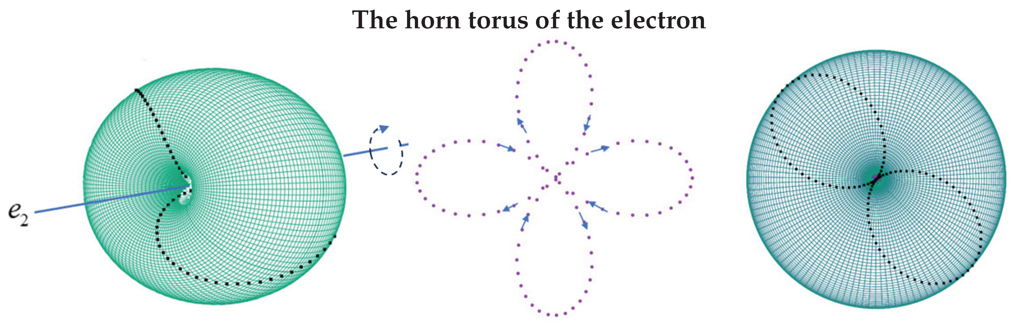
The major radius, , is the distance from the centre of the torus to the equatorial circle at , while the minor radius, , is the radius of the tube. Since the chord can shrink to zero length, we choose . This gives a horn torus where the inner hole closes and the surface pinches on the axis. There the chord has zero length. This geometry is illustrated in Figure 4. The torus represents all values of and , but the ZBW coordinate moves on the surface with a definite trajectory required by , also shown in Figure 4. It circles around at , while its radial distance from the axis oscillates at twice that rate. In particular, viewed down the axis, the chord lies in the plane that rotates, while its length oscillates between 0 and with frequency . It reaches its maximum, and breathes four times during each full rotation, returning to zero in between, Figure 4. Smoothly following the arrows of the center panel shows that for, say, left precession about the 2-axis, the petals move in and out sequentially in the opposite, right, direction.
From a multipole perspective, the four-petal rose is the natural symmetry once the rapid internal precession has averaged away all vector components. This leaves the lowest non-vanishing moment as a quadrupole. The four petals of the rose therefore represent the quadrupole projection of the dynamic bivector: four successive phases in which the internal chord expands and contracts in a state of even parity.
Toroidal Models
The geometrical picture that emerges from this analysis connects naturally with the long history of toroidal electron models. The earliest proposals began in 1915 with Parson’s ring-electron model [29], showing that circulating internal motion could account for its magnetic moment and angular momentum. Later ZBW-based approaches, especially the GA formulation of Hestenes [17], extended this idea by identifying an intrinsic circular motion as the origin of spin. Other constructions, such as helical-solenoid models of Consa’s [30] and EM-confined toroidal electrons proposed by Santos and Fleury, [31], have shown success.
A toroidal electron was proposed by Williamson and van der Mark, [32], who model the electron as a single photon confined on a double-loop torus of radius , the same as we find here. Their internal photon wavelength is equal to the Compton wavelength. They anticipate many features of the BSM, including real ZBW. What they lack is the geometric algebra framework needed to express their ideas consistently. The BiSM provides that missing structure. The torus becomes a bivector rotor; the double-loop topology becomes parity splitting; the circulating photon becomes the internal clock; and mass, spin, and interference emerge from a single confined bivector entity. The BiSM is not just close to the toroidal model, it provides its complete mathematical and physical basis.
A review by Fleury’s [33] emphasizes both the appeal and the limitations of these approaches. Across these areas, one sees the same underlying geometry: a two-dimensional internal plane supporting counter-rotating components whose projection into spacetime acquires a toroidal envelope. In the BiSM, this structure is not introduced by assumption, but naturally falls out of the geometry. The torus observed in the LFF does not require an extra hypothesis. The torus electron is not the starting point of a model but rather the consequence of spin being a bivector. This suggests why many disparate toroidal models have appeared over the past century and why the bivector offers the fundamental mechanism on which those models implicitly rely.
6. The Internal Clock
A clock is a physical system whose state evolves through a stable periodic cycle, allowing elapsed time to be measured by counting its cycles or fractions. The ZBW is direct evidence for such a real internal clock in the electron. In the BiSM this clock arises from the ontic cyclic motion of the bivector blades: their counter–precession fixes a definite instantaneous orientation in the 13-plane, just as the hands of a clock specify a moment of time. The dynamic chord then provides the projection of this internal time into the LFF. The clock does not arise from a quantization rule or from a superposition of energy eigenstates, but directly from the classical bivector structure.
de Broglie Wavelength
When the electron translates through space, the internal oscillation is carried forward with its motion. The internal phase that advances at the Compton rate in the BFF now accumulates along the electron’s trajectory in the LFF, giving the usual plane–wave form of the free electron,
Define the phase with and . At fixed time t the phase advances by when x increases by one de Broglie wavelength:
so that
Thus the de Broglie wave is a modulation of the internal Compton periodicity when the electron is transported through space. In this view, the de Broglie wavelength arises from the beat between the internal clock and the external translational motion. The bivector clock is, therefore, the origin of matter waves.
For reference, the de Broglie wavelength spans many orders of magnitude across common electron energies. A thermal electron at room temperature has , large enough to diffract from nanostructures, [34]. At , typical of low-energy electron diffraction, the wavelength shortens to about , comparable to atomic spacings, [35]. In electron microscopy, a beam has , well below the size of an atom, [36]. At relativistic energies, such as in transmission electron microscopes, the wavelength reaches the picometer scale, , far smaller than a Bohr radius, [37]. This rapid contraction of with increasing momentum reflects the geometrical modulation of the internal Compton clock that underlies matter-wave phenomena in the BiSM framework.
Although the modulation produces the standard plane–wave form in the LFF, there is no independent wave–particle duality in the BiSM. The internal rotor provides the localized, particle-like structure in the BFF, while the spatially accumulated phase of that same clock appears as the de Broglie wave in the LFF. The wave and particle descriptions are therefore complementary projections of a single bivector object rather than distinct physical modes of existence. The observed coherence and interference of matter waves arise directly from this geometrical structure and require no superposition of multiple states.
In summary, the internal clock acts as the heart of the electron, providing a stable geometrical rhythm inherent in the structure. It requires no external fields or adjustable parameters. It is the central physical ingredient of the bivector model. It supplies the ZBW, the torus, the spin properties, [3], and the de Broglie modulation. The clock emerges from the bivector and unifies the internal and external dynamics of the electron.
7. Discussion
In the BiSM, the LFF and the BFF are not two coordinate choices on a single spacetime manifold. They correspond to complementary parity sectors of the bivector. The LFF carries the odd-parity observable projection: an external rotating vector that couples to electromagnetic fields and enables measurement. The BFF carries the even-parity internal rotor formed by the counter-precessing blades; its dynamics result from conservative internal geometry of the electron.
A Lorentz transformation [6] acts entirely within Minkowski space. It preserves the metric, maps four-vectors to four-vectors, and preserves intrinsic parity. It cannot transport degrees of freedom into a different parity sector. Therefore no Lorentz boost or rotation can convert internal BFF variables (even parity) into LFF observables (odd parity). The relation between the two frames is not a coordinate transformation but a projection generated by the bivector rotor and its double cover. The BFFLFF correspondence is a geometrical transformations, not a map between relativistic inertial frames. This separation is not optional. The two frames possess distinct time generators: in the LFF and in the BFF. A Lorentz boost extended to the BFF would distort the internal clock, violating invariance of the Compton period. Maintaining separate time generators is therefore essential for consistency of the bivector structure.
Additional consequences follow from this complementarity. The EPR correlations [39,40] arise naturally when both the vector and bivector dynamics are taken into account. Bell’s inequalities [41] are violated not through nonlocality but through the presence of two distinct parity sectors, each of which provides correlation. The double cover is preserved, chirality of the blades is maintained, and spin acquires a dual structure consistent with the bivector geometry.
Within the BiSM, the ZBW is not an interference artifact but a real internal motion. Expressed in the BFF, the separation of the blades generates the internal ZBW chord. When projected to the LFF, this appears as a “twinkling” star. The resulting toroidal envelope follows directly from the geometry of the bivector motion and requires no additional assumptions. The torus is therefore not a model input but an unavoidable geometric consequence of the bivector dynamics. The ZBW emerges as the visible projection of a real, energy-conserving internal rotation. This demonstrates the classical correspondence between internal and external motion once the bivector structure is recognized.
We conclude that the point-particle electron of the SM must give way to a two dimensional bivector with internal dynamics. The bivector is the simplest structure beyond a point, and the BiSM provides a coherent replacement framework in which the internal and external dynamics of the electron are not imposed but arise naturally from classical geometry. This viewpoint offers a unified basis for reinterpreting spin, chirality, and charge within the bivector structure.
Appendix A. Derivation of the Zitterbewegung
This appendix summarizes the standard textbook derivation of ZBW for a free Dirac particle in the LFF. No assumptions from the BiSM are used. The presentation follows Thaller [9] and Greiner [10].
Appendix A.1. Dirac Equation and Hamiltonian Form
We begin with the free Dirac equation,
with metric signature and coordinates . Multiplying on the left by and using gives the Schrödinger form
where . Define the standard velocity matrices
so that .
Appendix A.2. Velocity Operator
In the Heisenberg picture, . Using , we obtain
and therefore
The operator has eigenvalues (i.e. ) which is a consequence of the anti-commutation, . These eigenvalues characterize the internal spinor structure of the Dirac field rather than the classical velocity of a point particle.
Appendix A.3. Evolution of the Velocity Operator
Appendix A.4. Position Operator and the ZBW
Since , integration gives
The last term is time independent and absorbed into the constant, ,
yielding the standard form,
The first term is the initial position; the second gives the uniform drift of the center of mass; and the third is the conventional expression for the ZBW term,
References
- Schrödinger, E. Über die kräftefreie Bewegung in der relativistischen Quantenmechanik. Sitzungsber. Preuss. Akad. Wiss 1930, 418–428. [Google Scholar]
- Sanctuary, B. Quaternion Spin. Mathematics 2024, 12, 1962. [Google Scholar] [CrossRef]
- Sanctuary, B. The Fine-Structure Constant in the Bivector Standard Model. Axioms 2025, 14, 841. [Google Scholar] [CrossRef]
- Dirac, P.A.M. The quantum theory of the electron. Proc. R. Soc. Lond. Ser. A Contain. Pap. A Math. Phys. Character 1928, 117, 610–624. [Google Scholar]
- Dirac, P.A.M. A Theory of Electrons and Protons. Proc. R. Soc. Lond. A 1930, 126, 360–365. [Google Scholar]
- Peskin, M.; Schroeder, D.V. An Introduction To Quantum Field Theory; Frontiers in Physics: Boulder, CO, USA, 1995. [Google Scholar]
- Doran, C.; Lasenby, J. Geometric Algebra for Physicists; Cambridge University Press: Cambridge, UK, 2003. [Google Scholar]
- David, G.; Cserti, J. General theory of ZBW. Physical Review B—Condensed Matter and Materials Physics 2010, 81(12), 121417. [Google Scholar] [CrossRef]
- Thaller, B. The dirac equation; Springer Science & Business Media, 2013. [Google Scholar]
- Greiner, W. Relativistic quantum mechanics; Springer Berlin Heidelberg, 1990; Vol. 3. [Google Scholar]
- Bjorken, J. D.; Drell, S. D.; Mansfield, J. E. Relativistic quantum mechanics; 1965. [Google Scholar]
- Schrödinger, E. Collected Papers on Wave Mechanics; Blackie & Son, London, 1928. [Google Scholar]
- Foldy, L. L.; Wouthuysen, S. A. On the Dirac theory of spin 1/2 particles and its non-relativistic limit. Physical Review 1950, 78(1), 29. [Google Scholar] [CrossRef]
- Barut, A. O.; Zanghi, N. Classical model of the Dirac electron. Physical Review Letters 1984, 52(23). [Google Scholar] [CrossRef]
- Rodrigues, W. A., Jr.; Vaz, J., Jr.; Recami, E.; Salesi, G. About zitterbewegung and electron structure. Physics Letters B 1993, 318(4), 623–628. [Google Scholar] [CrossRef]
- Hestenes, D. Spacetime physics with geometric algebra. American Journal of Physics 2003, 71(7), 691–714. [Google Scholar] [CrossRef]
- Hestenes, D. The zitterbewegung interpretation of quantum mechanics. Found. Phys. 1990, 20, 1213–1232. [Google Scholar] [CrossRef]
- Gerritsma, R. Quantum simulation of the Dirac equation. Nature 2010, 463, 68–71. [Google Scholar] [CrossRef]
- Blatt, M.; Roos, R.C. F. Quantum simulations with trapped ions. Nature Physics 2012, 8(4), 277–284. [Google Scholar] [CrossRef]
- J. Arrazola, I.; Pedernales, J. S.; Lamata, L.; Solano, E. Digital-analog quantum simulation of spin models in trapped ions. Scientific reports 2016, 6(1), 30534. [Google Scholar] [CrossRef]
- Dreisow, F.; Heinrich, M.; Keil, R.; Tünnermann, A.; Nolte, S.; Longhi, S.; Szameit, A. Classical simulation of relativistic Zitterbewegung in photonic lattices. Physical Review Letters 2010, 105(14), 143902. [Google Scholar] [CrossRef]
- Insulators, T. Dirac Dynamics in Waveguide Arrays: From Zitterbewegung to Photonic. Quantum Simulations with Photons and Polaritons: Merging Quantum Optics with Condensed Matter Physics 2017, 181. [Google Scholar]
- Rusin, K.; Zawadzki, T. M.W. Zitterbewegung (Trembling Motion) of Electrons in Graphene. In Graphene Simulation. IntechOpen; 2011. [Google Scholar]
- Ahrens, S.; Zhu, S. Y.; Jiang, J.; Sun, Y. Simulation of Zitterbewegung by modelling the Dirac equation in metamaterials. New Journal of Physics 2015, 17(11), 113021. [Google Scholar] [CrossRef]
- Chen, R. L.; Chou, Y. J.; Hwang, R. R. Photonic surface Dirac cones in reciprocal magnetoelectric metamaterials. Journal of Applied Physics 2025, 138(20). [Google Scholar] [CrossRef]
- LeBlanc, L. J.; Beeler, M. C.; Jimenez-Garcia, K.; Perry, A. R.; Sugawa, S.; Williams, R. A.; Spielman, I. B. Direct observation of zitterbewegung in a Bose–Einstein condensate. New Journal of Physics 2013, 15(7), 073011. [Google Scholar] [CrossRef]
- Goldstein, H. Classical Mechanics; Addison-Wesley Publishing Compangy, Inc.: Reading, MA, USA, 1950; ISBN 0-201-02510-8. [Google Scholar]
- Do Carmo, M. P. Differential geometry of curves and surfaces: revised and updated second edition; Courier Dover Publications, 2016. [Google Scholar]
- Parson, A. L. A magneton theory of the structure of the atom. In Smithsonian Miscellaneous Collections; 1915; Volume 65. [Google Scholar]
- Consa, O. Helical solenoid model of the electron. Progress in Physics 2018, 14(2), 80–89. [Google Scholar]
- dos Santos, C. A.; Fleury, M. J. A simple electromagnetic model of the electron. arXiv 2025, arXiv:2510.22384. [Google Scholar] [CrossRef]
- Williamson, J. G.; Van der Mark, M. B. Is the electron a photon with toroidal topology. In Annales de la Fondation Louis de Broglie; Fondation Louis de Broglie, January 1997; Vol. 22, No. 2, p. 133. [Google Scholar]
- Fleury, M. J.; Rousselle, O. Critical Review of Zitterbewegung Electron Models. Symmetry 2025, 17(3), 360. [Google Scholar] [CrossRef]
- Prasad, R. D.; Prasad, N. R.; Prasad, N.; Prasad, S. R.; Prasad, R. S.; Prasad, R. B.; Shaikh, A. D. A Review on Scattering Techniques for Analysis of Nanomaterials and Biomaterials. Engineered Science 2024, 33, 1332. [Google Scholar] [CrossRef]
- Held, G. Structure determination by low-energy electron diffraction—A roadmap to the future. Surface Science 2025, 754, 122696. [Google Scholar] [CrossRef]
- Ke, X.; Bittencourt, C.; Van Tendeloo, G. Possibilities and limitations of advanced transmission electron microscopy for carbon-based nanomaterials. Beilstein journal of nanotechnology 2015, 6(1), 1541–1557. [Google Scholar] [CrossRef]
- Egerton, R. F.; Watanabe, M. Spatial resolution in transmission electron microscopy. Micron 2022, 160, 103304. [Google Scholar] [CrossRef]
- Noether, E. Invariante Variations probleme. Gott. Nachr 1918, 235–257. [Google Scholar]
- Sanctuary, B. Spin Helicity and the Disproof of Bell’s Theorem. Quantum Rep. 2024, 6, 436–441. [Google Scholar] [CrossRef]
- Sanctuary, B. EPR Correlations Using Quaternion Spin. Quantum Rep. 2024, 6, 409–425. [Google Scholar] [CrossRef]
- Bell, J.S. On the Einstein Podolsky Rosen paradox. Phys. Phys. Fiz. 1964, 1, 195. [Google Scholar] [CrossRef]
Figure 1.
Left: A bivector in the BFF. The rotating frame relative to the LFF freezes the bivector motion. Helicity rotates the bivector about the 2-axis, perpendicular to the page. Shown is cw helicity on the left and ccw on the right. The 1 and 3 axes counter-precess at twice the frequency of the external vector motion. Right: As the 2-axis spins faster, cones develop about the 1 and 3 axes, which are mirror images and counter-precess in tandem. These two axes of opposite chirality form the left and right “hands’’ of the electron.
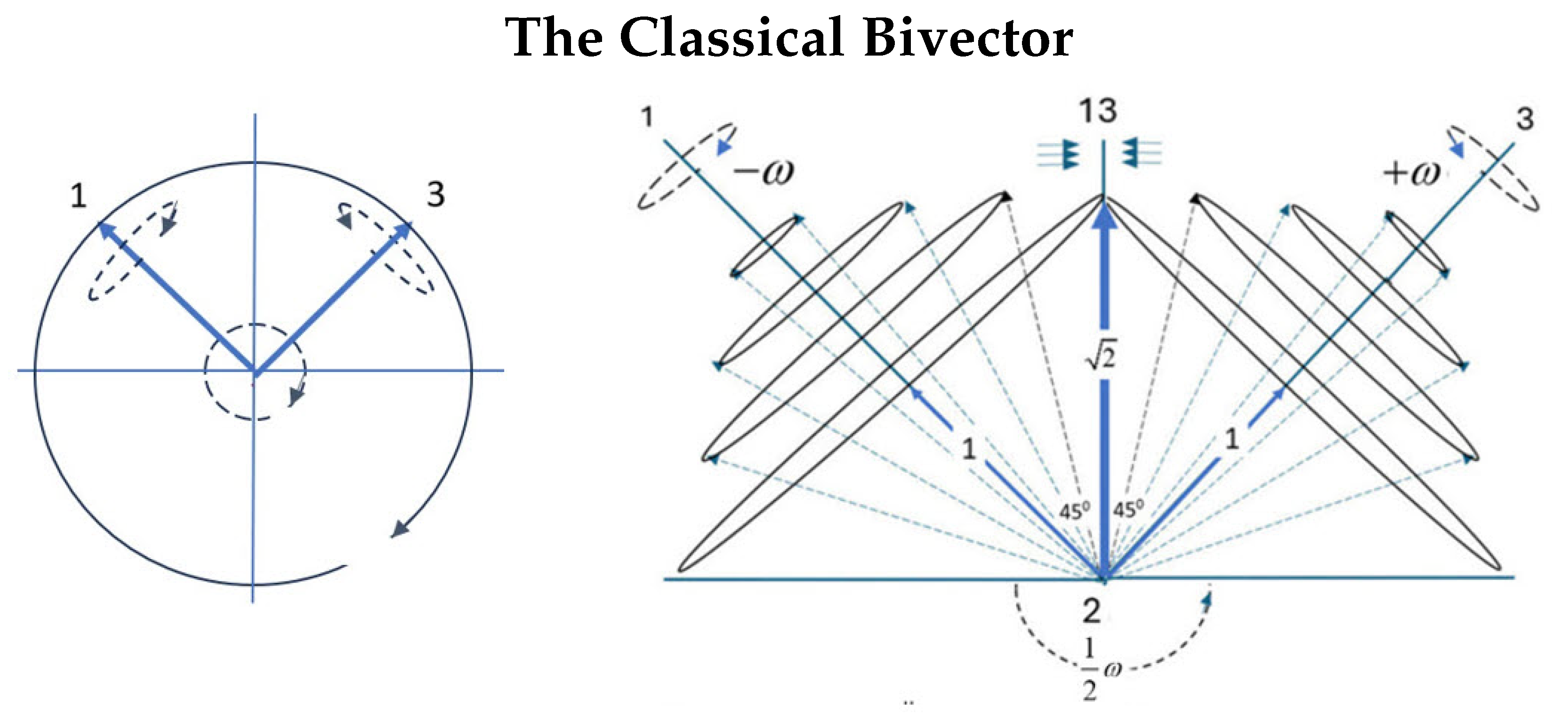
Figure 2.
Left: Dirac’s matter–antimatter pair of the SM. Right: The BiSM, showing two counter-precessing angular momentum cones on a single particle forming a bivector.
Figure 2.
Left: Dirac’s matter–antimatter pair of the SM. Right: The BiSM, showing two counter-precessing angular momentum cones on a single particle forming a bivector.
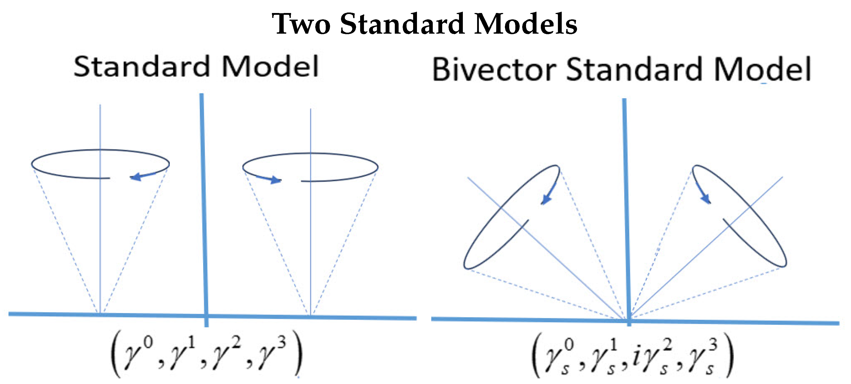
Figure 3.
The bivector as viewed down the torque axis, , showing the projection of the two precessing cones in the BFF. The angular momentum, and reflect each other. At closest approach, the angle between them is . As they precess, their oscillation is expressed by a time dependent chord, .
Figure 3.
The bivector as viewed down the torque axis, , showing the projection of the two precessing cones in the BFF. The angular momentum, and reflect each other. At closest approach, the angle between them is . As they precess, their oscillation is expressed by a time dependent chord, .
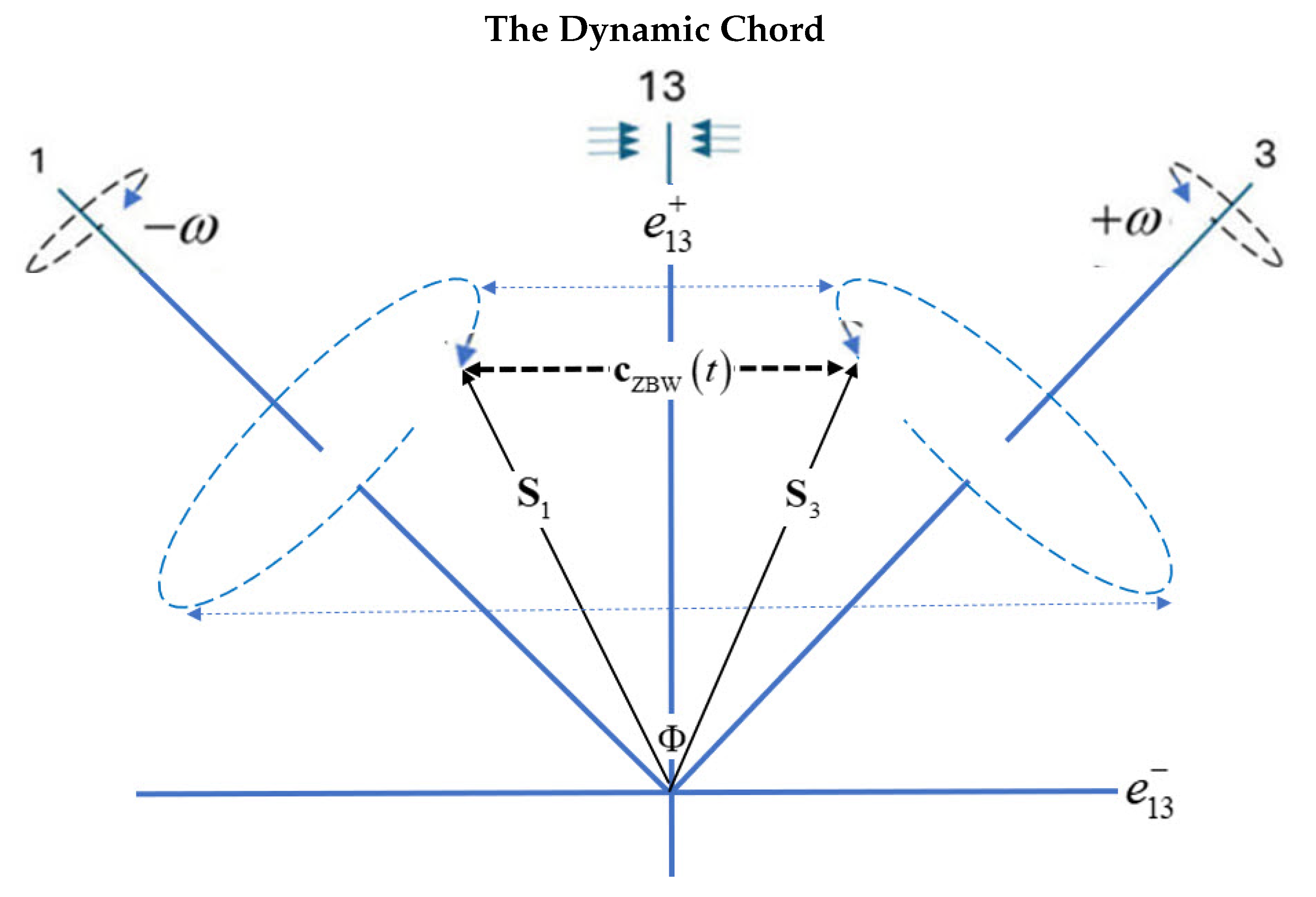
Figure 4.
The projection of the bivector dynamics into the LFF, giving a horn torus. Left: The torus is centred on the axis, and the dashed curve on the torus shows how the length of the internal chord varies as it loops around the torus. Right: View same along the axis. Centre: The sequence of points represents the instantaneous chord length plotted in polar coordinates. As the internal phase advances, the chord expands to the tip of a petal and then contracts back to the origin before the next petal begins. Following the arrows shows that the four petals correspond to four successive breathing cycles of the torus in one period.
Disclaimer/Publisher’s Note: The statements, opinions and data contained in all publications are solely those of the individual author(s) and contributor(s) and not of MDPI and/or the editor(s). MDPI and/or the editor(s) disclaim responsibility for any injury to people or property resulting from any ideas, methods, instructions or products referred to in the content. |
© 2025 by the authors. Licensee MDPI, Basel, Switzerland. This article is an open access article distributed under the terms and conditions of the Creative Commons Attribution (CC BY) license (http://creativecommons.org/licenses/by/4.0/).
Copyright: This open access article is published under a Creative Commons CC BY 4.0 license, which permit the free download, distribution, and reuse, provided that the author and preprint are cited in any reuse.


