
Submitted:
05 December 2025
Posted:
05 December 2025
You are already at the latest version
Abstract
A sustainable city requires a sustainable means of transportation. This ambition is leading towards a higher penetration of electric vehicles (EVs) in our cities, in both the private and commercial sectors, putting more and more burden on the existing power grid. Modern deregulated power grids vary electricity tariffs from location to location and from time to time, to compensate for any additional burden. In this paper, we propose a profit-aware solution to strategically manage the movements of EVs in the city to support the grid while exploiting these locational, time-varying prices. This work is divided into three parts: M1) Profit-aware charging location and optimal route selection, M2) Profit-aware charging & discharging location and optimal route selection, and M2b) Profit-aware charging & discharging location and optimal route selection considering the demand-side flexibility. This work is tested on the MATLAB programming platform using the Gurobi optimisation solver. From the extensive case study, it is found that M1 can yield profits up to 2 times more than those of its competitors, whereas M2 can achieve profits up to 2.5 times higher and simultaneously provide substantial grid support. Additionally, M2b extension has made M2 more efficient in terms of grid support.
Keywords:
electric vehicle
; sustainability
; smart cities
; route selection
; charging station selection
; vehicle-to-grid
; power grid
; city grid mapping
1. Introduction
The rapid adoption of electric vehicles (EVs) is a cornerstone in the evolution of sustainable smart cities. In 2024, global EV sales reached approximately 17.1 million units, marking a 25% increase from the previous year1. EVs now account for more than 20% of new car sales worldwide, underscoring a significant transition toward cleaner urban mobility and energy systems.However, the benefits of EVs can only be fully realized if charging infrastructure and management strategies evolve in parallel. Today, most EV charging is uncoordinated and often concentrated during peak hours, which amplifies grid demand spikes. High-power consuming charging stations in particular draw substantial loads, creating localized imbalances. With millions of additional charging points projected worldwide, the implications for land use, grid reinforcement, and local reliability are significant. However, coordinated and smart charging can transform EVs from potential burdens into distributed storage assets that enhance renewable integration and grid resilience [1].
Smart charging and bidirectional vehicle-to-grid (V2G) operations are emerging as transformative solutions. Smart charging shifts demand to off-peak periods or aligns charging with renewable availability, while V2G enables EVs to discharge power back to the grid at times of high demand [2]. Together, these strategies allow EVs to integrate renewables, mitigate peak demand, and provide ancillary services. Yet, their widespread deployment introduces challenges such as voltage fluctuations, transformer stress, and rising system peaks [3].Case studies highlight the complexity of EV integration. An energy management research on microgrids demonstrates that EVs can reduce costs by nearly half while improving resilience [4]. Another work on DC microgrid prototype confirms that optimal EV control can stabilize power flows and lessen dependence on the main grid [5]. At the city level, synergies between EVs and metro systems in Madrid illustrate how regenerative braking energy can be captured and stored in EV batteries [6]. Further examples from Valencia emphasize that effective policy, financial incentives, and infrastructure readiness are decisive in overcoming adoption barriers [7].
These studies also show that while technical and environmental considerations are crucial, economic incentives remain the key enabler of large-scale adoption. Without clear financial benefits, such as savings from time-variable tariffs or efficient use of demand response incentives, advanced charging schemes may see limited uptake.This paper proposes a profit-aware utilization framework for EVs in sustainable smart cities. The framework integrates profitability for EV owners with grid stability and urban sustainability goals, leveraging a strategic optimization approach that accounts for locational and time-varying electricity prices. By this approach, the proposed models position EVs not merely as clean transportation options but as economically sustainable energy assets within the city.
1.1. Literature Review
The role of EVs in smart cities and sustainable energy systems has been studied extensively, with growing emphasis on smart charging, bidirectional V2G operations, and route optimization. This section reviews recent contributions in three directions: smart charging, charging and discharging with grid impacts, and route optimization.
EV Smart Charging: Uncoordinated charging, where EVs begin charging immediately upon plug-in, raises peak demand and stresses distribution assets. Smart charging coordinates charging with electricity prices, renewable generation, or grid constraints to enhance performance. On the behavioral side, Barman et al. [8] introduced a random utility model that jointly captures travel and charging choices, offering greater realism than simplified assumptions. Operational methods focus on cost, waiting time, and travel delay: ant colony optimization reduced both waiting times and charging expenses [9], while centralized fleet scheduling improved peak demand reduction and PV utilization compared to uncoordinated strategies [10]. Reinforcement learning has also gained traction; Sultanuddin et al. [11] showed that Double Deep Q-learning reduced load variance by 68% relative to uncontrolled charging. Renewable integration studies further demonstrate that workplace PV-EV systems improve renewable utilization by more than 40% under the self-consumption-sufficiency balance (SCSB) metric [12].
Charging and Discharging with Grid Impact: While smart charging primarily addresses charging load management, recent work extends to the dual role of charging and discharging. Zheng and Yao [13] proposed a multi-objective allocation method for PV-based stations, showing that orderly V2G reduces both grid stress and costs. Tian et al. [14] developed a two-stage optimization for distribution systems that improves stability and efficiency. Shaheen et al. [15] demonstrated that metaheuristic methods generate cost-effective V2G schedules that also deliver ancillary services. Reinforcement learning methods, such as recurrent proximal policy optimization with LSTM forecasting, balance supply-demand under uncertainty [16]. These approaches highlight the resilience potential of V2G, though most remain system-level rather than mobility-aware.
At the distribution scale, Abiassaf et al. [17] showed that unmanaged large-scale EV adoption leads to voltage instability, transformer overloading, and congestion, particularly with fast charging. Optimized charging integrated with renewables mitigates these issues. Urban-level studies, such as Khalid et al. [18] on Stockholm’s grid, show that coordinated charging reduces congestion and losses, and that PV and BESS integration further enhance outcomes. Microgrid studies add stochastic realism: Iqbal et al. [19] used Markov-based scheduling to account for travel variability, achieving cost-effective V2G while preserving mobility. Reliability-focused studies caution against unmanaged charging; Roy et al. [20] found accelerated transformer degradation under high EV penetration in rural Kentucky.
Route Optimization with Charging and Discharging: As EV deployment accelerates, charging and discharging decisions along routes are increasingly embedded into routing models. Algafri et al. [21] proposed an optimization model for station allocation while doing G2V/V2G transactions, achieving over 85% satisfaction for charging and nearly 99% for discharging requests. Long-distance travel studies across Germany confirmed that charging requirements increase average travel time by 8%, with poor station distribution causing delays up to 30% [22], underscoring the importance of spatial planning. Advanced formulations explicitly capture nonlinear charging: Kim et al. [23] showed that ignoring state-of-charge dependencies yields infeasible routes, while Shahkamrani et al. [24] combined route mapping with day-ahead optimization to reduce network losses by 25%.
Overall, the literature demonstrates strong advances in smart charging, V2G scheduling, and routing optimization. Yet, most studies consider charging or routing in isolation, overlooking the strategic joint optimisation over EV charging and discharging opportunities, power grid’s locational and temporal price variations, and city road’s connections and distances along a trip. Addressing this limitation is crucial to transform EVs into profit-aware, mobility-integrated energy assets, supporting both user incentives and urban grid stability in sustainable smart cities.
1.2. Motivations
The growing adoption of EVs in both private and commercial sectors is a key driver of sustainable urban mobility, yet it places increasing stress on existing power grids. In deregulated markets, electricity tariffs fluctuate across locations and time periods, adding further complexity to EV charging and discharging decisions. While these dynamics help balance grid demand, they create economic and operational challenges for EV owners, fleet operators, and urban planners.
Although prior studies have explored smart charging, V2G-enabled discharging, and routing optimization, most approaches treat these aspects separately. As a result, opportunities to align profitability with grid stability and sustainability remain underutilized. This gap motivates the need for an integrated, profit-aware framework that strategically combines routing with charging and discharging decisions. By leveraging locational and time-varying prices, EVs can evolve from clean transport modes into active energy assets, supporting both urban mobility and resilient power systems.
1.3. Contribution
- A profit-aware EV utilisation model (PAUM-EV-M1) is developed for charging location and optimal route selection for conventional EVs;
- A profit-aware EV utilisation model (PAUM-EV-M2) is developed charging–discharging location and optimal route selection for V2G-enabled EVs;
- Extended the PAUM-EV-M2 models (PAUM-EV-M2b) to work under the flexibility and uncertainty of demand-side resources.
2. Profit-Aware Electric Vehicle Utilisation Model (PAUM-EV)
In this section, three different models are proposed in which EVs are optimally utilised along with other flexible loads to attain higher profits without imposing infeasible burdens on the grid. Here, the decision-making process is managed by the utility-owned (of affiliated) aggregator that has real-time access to various operational parameters of the city’s power distribution network. EV users participate in this process through a mobile application and provide the necessary inputs; other fixed details are collected during the application registration. Depending on the available time and technical feasibility, EV users may opt between smart charging (M1) or smart charging and discharging (M2) methods. Based on the selected options and surrounding possibilities, the aggregator chooses the objective and associated constraints to obtain the solutions.
2.1. Proposed PAUM Objective Function
The objective function in Eq. (6) has three operational factors (Eq. 1,,) and two profit-related factors (Eq. ,). Three operation factors include one optional DSM factor (Eq. ). These factors are described mathematically as follows:
All factors are normalised by dividing with respective maximum feasible values, as denoted by to . The also used as a binary switch to turn on or off the demand management ability. These five factors are arranged in objective functions as follows:
Here, deals with error between EVs’ demanded energy and aggregator’s caterable energy; deals with selecting charger location; and deal with energy cost payable to grid and battery degradation cost on EV users; finally, deals with amount of demand need to be curtailed to optimise the overall cost and feasibility. The entire proposed PAUM model, including Eq. (6), is solved for three categories of decision variables, viz. power grid-related variables (PGV), city grid-related variables (CGV), and EV-related variables (EVV), as discussed in the models in the following subsections.
2.2. PAUM Systems Modelling
The entire PAUM framework consists of three major systems: the EV system, the CG system, and the PG system. In the following subsections, the mathematical models for each system are presented, and the system interconnections are explained. In the later sections, their curated applications are elaborated.
2.2.1. EV System Model
If the is the energy level of the EV , and and are the associated charging and discharging powers in the EV, respectively, then decisions on all three variables for time t and for the multiple EV system can be evaluated by solving the following mathematical models:
Here, the battery capacity and SoC of the EVs are not explicitly modelled rather internalised here as energy levels of the EVs. If the model converged, we move to the next time instance . Then, the obtained decisions are stored for next t as , , , and .
In this EV system model, Eq. (7) establishes the relationship between the battery energy level and the charging and discharging powers. Eq. (8), (9), and (10) impose limitations on the energy level, as well as the charging and discharging powers, respectively. Eq. (11) and (12) ensure the timely fulfilment of the energy needs. The energy fulfilment errors are evaluated by Eq. (12), (13), and (14). Finally, the constraints specified in Eq. (15) are utilised for model predictive control (MPC) enforcement.
2.2.2. PG System Model
Power grid (PG) system is modelled using the bus voltage (V) limits, angle () limits, real power generation () limits, load () limits, and lines flow () limits. Here, the power flow equation along with parameter limitations are mathematically expressed in its polar form, as follows:
Here, the power balance equation for fixed non-elastic PG bus loads and flexible EV loads are modelled as follows:
Along with charging (C) and discharging (D) of EVs, this model also governs the decision of charging station location (L) on the grid. This can be made 0 for the buses without any charging stations connection. Note that the impact of reactive power is not taken into account, as we are focusing on energy-related evaluations.
2.2.3. CG System Model
In this study, the city’s road infrastructure is modelled as a grid-like graph , where each junction is equated with vertices and connecting roads are equated with edges. The distance of the road is presented on as weights on the edges. Please refer to Figure 1 and Figure 3 for better illustration. In the graph, the minimum distance between source and destination nodes ( and ) is evaluated using Dijkstra algorithm [25]. The decision vector L with two identical indices l and b is used map presence of EV charging stations on both CG and PG. Furthermore, mapping of PG on to the CG is also supported by the variables , as discussed in Sec. Section 2.5.
The primary constraints in the CG system deals with , i.e. time required to travel over a shortest distance between two points v and . These are modelled as:
Here, indicates the nearest node on the city grid from where the EV user has started the M.App. is factor that converts the distance in kilometer to approximate time in hours, neglecting the traffic congestion. In the CG system, Eq. (22) defines the parameter . Eq. (23) and (24) implement the reach time feasibility on to the EV’s initial energy level and charging start time. Eq. (25) imposes the minimum distance restriction on decision-making process using to avoid assignment of a distant charger. Finally, Eq. (26) enforces the MPC and commitment continuity on the EVCS location selection variables.
2.3. PAUM-EV-M1: Profit-Aware Charging Location and Optimal Route Selection
In this model (M1), only the charging requirements of EVs are considered, making it suitable for a city without provisions for EV discharging or for EVs that are not designed to discharge. When EV user starts the M.App, the aggregator collects the current battery level and current location of the EV in the city-grid. Then, the EV user manually fill out the M.App with his final destination on the city-grid and desired time to reach there. The aggregator has the prior knowledge on CG map, PG map, CG—PG connecting maps and the location of EV charging stations on those maps. Now, Aggregator solves the PAUM-EV optimisation models as shown in Figure 2.
To consider only charging but not discharging, we slightly update the Eq. (7), (9), and (10) as follows:
Here, energy level inside the EV does not change due to discharging and does not go to negative; only keeps increase until departure. Hence, the key goal became to find the appropriate EVCS location and the charging schedule given other EV, CG and PG system constraints are satisfied. To do this, we minimise the objective function in Eq. (6) and solves the constraints in Eq. (8), (11)–(15), (16)–(21), (22)–(26), (27)–(29),
2.4. PAUM-EV-M2: Profit-Aware Charging–Discharging Location and Optimal Route Selection
For a favourable situation, where the city has EV discharging provision and EVs have V2G enabled battery management system, this model M2 can be deployed. Here, the EV system models in Eq. (7)–(15) is fully restored, the discharging of EV can go from 0 to its minimum () value and similarly, charging can span freely between 0 to , as presented below:
Furthermore, unlike charging the discharging efficiency gets divided, as EV has to discharge more ,i.e. , for the grid to get certain amount of energy . To operate in this model M2, aggregator minimise Eq. (6) while adhering to the EV, PG, and CG system models and limitations in Eq. (7)–(15), (16)–(21), (22)–(26).
2.5. PAUM-EV-M2b: Extension of PAUM-EV-M2 Considering the Demand Flexibility
Finally, having proposed a method to deal with EV charging and discharging in PAUM-EV-M2, we extended the model in PG systems to appropriately manage the flexible loads in the city, as follows:
Here, the demand management variable is continuous and can be defined as:
The electrical loads distributed across the city grid is usually have the connections from the nearest electrical bus, any deviation can be mapped on and decisioned with .
3. Results and Discussions
3.1. Simulation Set-Up
The primary focus of this research is to obtain a holistic and optimal solution through the joint optimisation of EV system, power grid system, and city’s road grid system. Information on these three systems are collected as follows:
- The EV arrival and departure time and energy level, battery capacity and efficiency information are availed from the dataset referred in [26].
- Power grid system information, such as power generation, non-elastic load, and radial distribution line topology are collected from the IEEE 33 Bus system data [27].
- City’s road grid information is derived from an check-board pattern city, like Manhattan in New York, where each junction (graph vertices) is approximately equidistantly placed. In the present study, the graph edge weight is assumed to be 5km uniformly, shown in Figure 1. It can easily be extended to non-uniform weights as shown in Figure 3.
Effectiveness of the proposed profit-aware EV utilisation models are tested on a workstation with 16GB RAM and Intel-i5 11th Gen 2.40GHz processor using MATLAB programming platform and Gurobi optimisation solver.
The CG and PG interconnection mapping information is presented in a supplementary sheet in [28]. Figure 4 presents the equidistantly installed EV charging stations in the city, which is used in the case studies. In the Figure 5, arrival and departure locations of the 30 EVs (mentioned as per the sequence in [26]) are depicted. Figure 6 illustrates the PG system and its mapping on to the CG system. It highlights the jurisdiction of the aggregator on the IEEE 33 bus system, and shows how the lines and buses are spread across the CG system covering the load centers in the city. In this interconnected mapping, it is assumed that each bus in the PG system supplies all electrical loads in the CG squares surrounding it, extending to the road on the right and the road above. Note that the civil infrastructure issues and traffic considerations are not considered in this research.
Figure 3.
Central region of Singapore, a non-check-board pattern city, where similar to Manhattan junctions can be presented as vertices and roads connecting them can be presented as edges. However, the weights of these edges are going to be very dissimilar in this case.
Figure 3.
Central region of Singapore, a non-check-board pattern city, where similar to Manhattan junctions can be presented as vertices and roads connecting them can be presented as edges. However, the weights of these edges are going to be very dissimilar in this case.
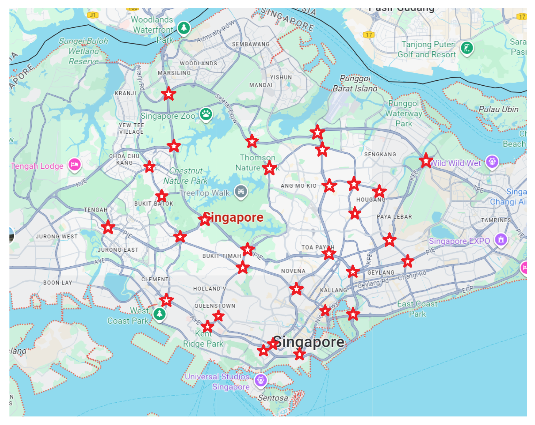
Figure 4.
Illustration of a smart city’s graph-based road grid infrastructure and equidistantly placed of EV charging stations (indicated with red square dots). Gray lines and dots indicate roads and junctions, respectively. The numbers in x-axis and y-axis are used to mark any node and line.
Figure 4.
Illustration of a smart city’s graph-based road grid infrastructure and equidistantly placed of EV charging stations (indicated with red square dots). Gray lines and dots indicate roads and junctions, respectively. The numbers in x-axis and y-axis are used to mark any node and line.

Figure 5.
Illustration of EV’s initial (left) and destination (right) locations, indicated with down and up triangles, respectively. The numbers indicate the EV numbers as sequenced in [26].
Figure 5.
Illustration of EV’s initial (left) and destination (right) locations, indicated with down and up triangles, respectively. The numbers indicate the EV numbers as sequenced in [26].
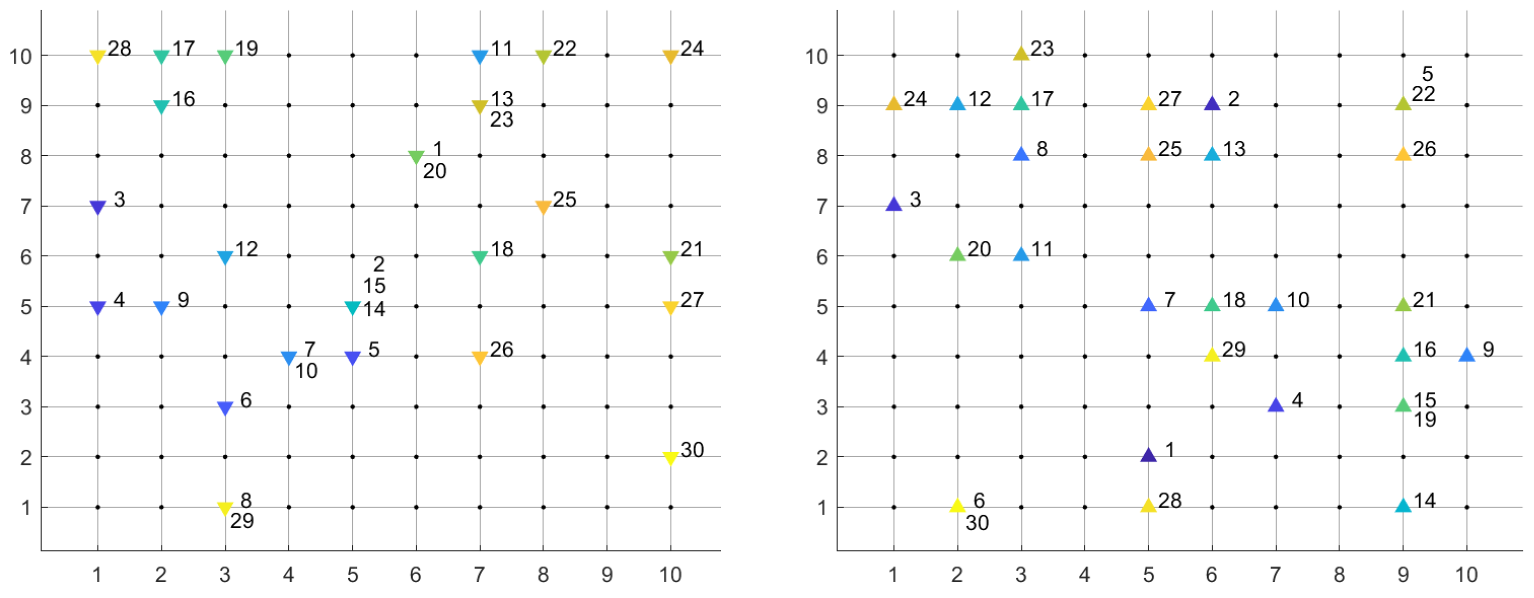
Figure 6.
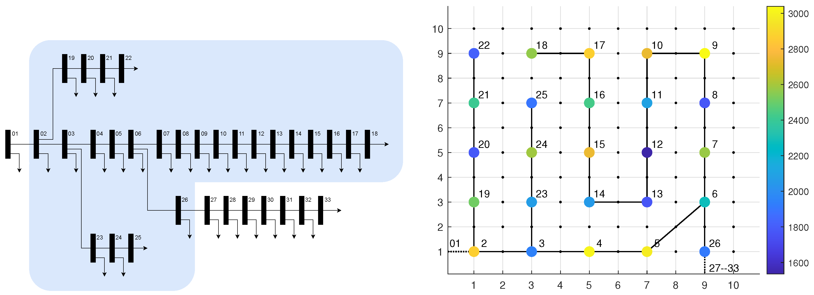
(Left) Single line diagram of IEEE 33 bus system; shaded region indicates the buses within the aggregator’s jurisdiction (i.e. within the city) and the remaining buses are within the larger urban system but beyond the aggregator’s control. (Right) An illustrative mapping of the 25 buses in the radial IEEE 33 bus system onto the city’s road grid system, including their bus connection topology.
Figure 6.
(Left) Single line diagram of IEEE 33 bus system; shaded region indicates the buses within the aggregator’s jurisdiction (i.e. within the city) and the remaining buses are within the larger urban system but beyond the aggregator’s control. (Right) An illustrative mapping of the 25 buses in the radial IEEE 33 bus system onto the city’s road grid system, including their bus connection topology.
In all the case studies, the real-time prices (RTPs) from Singapore’s wholesale market, based on the NEMS database’s October 2024 data [29], are used. Since the available sample rate in NEMS is 30 min, we have considered two days information to portray as 15 minute interval for 24 hours (96 samples). Furthermore, this RTPs (say ) do not reflect the generation and demand mismatch in our case study, rather was cleared in the market for a very bids. Hence, to reflect the actual load imbalance in the nodes in the city, we converted the for individual nodes in the PG as follows:
If any nodal price is found to be negative, an offset value may also be added by deriving the absolute of minimum of , .
This mechanism prepares different for different buses , which now represent the true imbalance in the grid. In this paper, market clearing process is not the primary focus; in a real world scenario, Eq. (32) can be replaced with market cleared LMP prices.
3.2. Case-1: Charging Schedule of EV, EVCS Location and Route Selection
In this case study, we have primarily assessed the performance of PAUM-EV-M1 in three different systems. In Figure 7(a), the nodal and temporal price variation including the imbalance factor (as discussed in Eq. 32) is presented as colourmap. Its impact on the driver route selection is illustrated in Figure 7(b). As can be noticed, traditional drivers pricked the most nearest EVCS location and the route (the green line) that is not far from his envisaged travelling route (the blue line), despite their higher nodal prices.
On the contrary, when we consider PAUM-EV-M1 in its full potential along with the restructured nodal prices, the profits are visible. EV optimally choosed a slightly longer route (the brown line) and a distant EVCS, biased by the lower nodal prices, but managed to obtain a significant profit compared to the traditional strategy, as shown in Figure 8.
In Figure 8, four items are presented, namely, cost, distance, time and schedule, and are compared between the traditional charging strategy (without the profit consideration) and the proposed PAUM-EV-M1 strategy. As can be noticed from Figure 8(a) and (b), the financial benefits of EV owners are significantly higher with proposed model, approximately $260. On the contrary, the increase in travel distance ( Figure 8(c) & (d)) and time ( Figure 8(e) & (f)) are around 90km and 17 minutes, respectively.
Other than the selection of the optimal EVCS nodes, another major reason behind this financial benefit can be understood by analysing the temporal variation of nodal prices and the charging schedules in Figure 8(g) & (h). Contrast to the traditional charging strategy, where EV is getting the required charge continuously as soon as it is coming to the station, in the proposed model, charging is done strategically when price is low and the EV stays idle when prices are high. But, in this process of cost reduction, the model did not ignore the EVs energy requirements. Furthermore, the initial flat pricing periods indicate the moment EV initiated the M.App vs the moment EV’s charging initiated. Some EVs exhibit partial charging owing to their small stay duration.
In this case study, we are assessing the performance of PAUM-EV-M2 strategy, that focuses on both strategic charging and discharging. It is also compared against PAUM-EV-M1 strategy and traditional charging strategies capable of doing discharging to minimise overall objective cost-function. The obtained results are presented Figure 9 in four terms, i.e., cost, distance, reach time, and schedules.
As can be noticed in Figure 9(a) & (b), the financial benefit with the proposed PAUM-EV-M2 is $390 higher than the traditional strategy. Furthermore, the benefit is better than just smartly charging with M1; in this case study, it is found to be around $80. The key reason behind this better performance is the strategic decision to discharge back to the grid (V2G process) when the price is high, which is visible in Figure 9(g) & (h). In the traditional strategy is discharging is happening to compensate other system objectives, but ignores the sole financial benefit of the EV users. On the other hand, by analysing the charging and discharging schedules of EVs with temporal price variations, we can notice that the energy discharge is happening during the high price time and charmings are done during low price hours.
Moreover, similar to M1, the distance covered by EVs ( Figure 9(c) & (d)) and reach time of EVs ( Figure 9(e) & (f)) is slightly higher in M2 compared to the traditional strategy; however, they remained nearly equal in M2 when compared with the M1.
Hence, looking at the financial benefits, it is advisable for the EV users to opt for the PAUM-EV-M2 model if the charging station and the EV has the technical feasibility to discharge back.
3.4. Case-3: Charging and Discharging Schedules Along with Demand Management
Finally, in this case study, we analysed the performance of the extension of the PAUM-EV-M2 model (say M2b model) by incorporating the impact of the flexible demand management. The impact is presented in the Table 1.
Since the EV utilisation is also burdened by the power grid system constraints, sometimes EV systems may experience additional adjustments in charging and discharging schedules to support this. These constraints are essential for grid stability and can not be relaxed. Hence, to reduce the extra burden on the EV system, flexible demands in the power grid systems are optimally reduced, as can be noticed in the table.
Note that, in this research, a very approximated power grid constraints are utilised, which can be extended in future for a more detailed modelling.
Hence, if it is technically feasible in the power grid system to initiate flexible load management, by combining this with the EV utilisation model can be significantly beneficial for power grid system as well as EV systems, and will contribute towards city’s sustainability goals.
4. Conclusions and Future Works
In this paper, three profit-aware EC utilisation models are proposed to enhance the challenges in sustainability goals of a city. In this context, a joint optimisation strategy is developed over three different inter-related systems, namely, EV systems, power grid systems, and city grid systems. From a several case studies over a combination of real-world and synthetic datasets, following key conclusions are observed:
- Both M1 and M2 can yield more profit for EVs compared to their traditional counterparts, e.g. $260 and $390 in this case, while doing a minimum re-routing of the EVs. M2 is capable of obtaining better financial benefits than M1 (around $80), but it is subjected to technical feasibility at the EV and EVCS end.
- The enhanced model M2b, flexible demand management can further contribute towards reducing the kW burden on the power grid across the city by optimally balancing the flxible loads subject to EV charging burden and price structure.
- Contrast to the traditional EV charging strategies, the proposed M1 and M2 model focuses on the both aspects of the price structure in the city, namely, the nodal variations and the temporal variations. This makes the proposed model more profit oriented compared to the traditional models, more grid requirement aware, and hence, a better alternative to accomplish the sustainable city goals.
In future, we will study more in-depth modelling with the city’s traffic structure, and will do an analyse societal constraints on the flexible demand management.
Nomenclature
| Abbreviations | |
| EV | Electric Vehicle |
| CG | City Grid (System) |
| PG | Power Grid (System) |
| M. App | Mobile Application |
| RTP | Real-Time Pricing |
| PAUM | Profit-Aware Utilisation Model |
| PAUM-EV | Profit-Aware EV Utilisation Model |
| V2G | Vehicle-to-Grid |
| FDM | Flexible Demand Management |
References
- Reddy, K.; Kumar, M.; Mallick, T.; Sharon, H.; Lokeswaran, S. A review of Integration, Control, Communication and Metering (ICCM) of renewable energy based smart grid. Renewable and Sustainable Energy Reviews 2014, 38, 180–192. [Google Scholar] [CrossRef]
- Wouters, H.; Martinez, W. Bidirectional onboard chargers for electric vehicles: State-of-the-art and future trends. IEEE Transactions on Power Electronics 2023, 39, 693–716. [Google Scholar] [CrossRef]
- Astapov, V.; Shabbir, N.; Rosin, A.; Kütt, L.; Maask, V.; Tiismus, H. Review of technical solutions addressing voltage and operational challenges in a distribution grid with high penetration of intermittent RES. Energy Reports 2025, 14, 1738–1760. [Google Scholar] [CrossRef]
- Jiang, J.; Li, Y.; Li, Y.; Li, C.; Yu, L.; Li, L. Smart transportation systems using learning method for urban mobility and management in modern cities. Sustainable Cities and Society 2024, 108, 105428. [Google Scholar] [CrossRef]
- Marino, P.; Rubino, G.; Rubino, L.; Capasso, C.; Veneri, O.; Motori, I. A case study of a DC-microgrid for the smart integration of renewable sources with the urban electric mobility. In Proceedings of the 2018 International Symposium on Power Electronics, Electrical Drives, Automation and Motion (SPEEDAM); IEEE, 2018; pp. 544–549. [Google Scholar]
- Calvillo, C.F.; Sánchez-Miralles, Á.; Villar, J. Synergies of electric urban transport systems and distributed energy resources in smart cities. IEEE Transactions on Intelligent Transportation Systems 2017, 19, 2445–2453. [Google Scholar] [CrossRef]
- Bastida-Molina, P.; Ribó-Pérez, D.; Gómez-Navarro, T.; Hurtado-Pérez, E. What is the problem? The obstacles to the electrification of urban mobility in Mediterranean cities. Case study of Valencia, Spain. Renewable and Sustainable Energy Reviews 2022, 166, 112649. [Google Scholar] [CrossRef]
- Barman, P.; Dutta, L.; Bordoloi, S.; Kalita, A.; Buragohain, P.; Bharali, S.; Azzopardi, B. Renewable energy integration with electric vehicle technology: A review of the existing smart charging approaches. Renewable and Sustainable Energy Reviews 2023, 183, 113518. [Google Scholar] [CrossRef]
- Moghaddam, Z.; Ahmad, I.; Habibi, D.; Phung, Q.V. Smart Charging Strategy for Electric Vehicle Charging Stations. IEEE Transactions on Transportation Electrification 2018, 4, 76–88. [Google Scholar] [CrossRef]
- Huang, P.; Munkhammar, J.; Fachrizal, R.; Lovati, M.; Zhang, X.; Sun, Y. Comparative studies of EV fleet smart charging approaches for demand response in solar-powered building communities. Sustainable cities and society 2022, 85, 104094. [Google Scholar] [CrossRef]
- Sultanuddin, S.; Vibin, R.; Kumar, A.R.; Behera, N.R.; Pasha, M.J.; Baseer, K. Development of improved reinforcement learning smart charging strategy for electric vehicle fleet. Journal of Energy Storage 2023, 64, 106987. [Google Scholar] [CrossRef]
- Fachrizal, R.; Shepero, M.; Åberg, M.; Munkhammar, J. Optimal PV-EV sizing at solar powered workplace charging stations with smart charging schemes considering self-consumption and self-sufficiency balance. Applied Energy 2022, 307, 118139. [Google Scholar]
- Zheng, X.q.; Yao, Y.p. Multi-objective capacity allocation optimization method of photovoltaic EV charging station considering V2G. Journal of Central South University 2021, 28, 481–493. [Google Scholar] [CrossRef]
- Tian, P.; Yan, S.; Pan, B.; Shi, Y. Two-stage optimization for efficient V2G coordination in distribution power system. In Proceedings of the 2024 IEEE International Conference on Communications, Control, and Computing Technologies for Smart Grids (SmartGridComm); IEEE, 2024; pp. 245–251. [Google Scholar]
- Shaheen, H.I.; Rashed, G.I.; Yang, B.; Yang, J. Optimal electric vehicle charging and discharging scheduling using metaheuristic algorithms: V2G approach for cost reduction and grid support. Journal of Energy Storage 2024, 90, 111816. [Google Scholar] [CrossRef]
- He, C.; Peng, J.; Jiang, W.; Wang, J.; Du, L.; Zhang, J. Vehicle-To-Grid (V2G) Charging and Discharging Strategies of an Integrated Supply–Demand Mechanism and User Behavior: A Recurrent Proximal Policy Optimization Approach. World Electric Vehicle Journal 2024, 15, 514. [Google Scholar]
- Abiassaf, G.A.; Arkadan, A.A. Impact of EV charging, charging speed, and strategy on the distribution grid: a case study. IEEE Journal of Emerging and Selected Topics in Industrial Electronics 2024, 5, 531–542. [Google Scholar] [CrossRef]
- Khalid, M.; Thakur, J.; Bhagavathy, S.M.; Topel, M. Impact of public and residential smart EV charging on distribution power grid equipped with storage. Sustainable Cities and Society 2024, 104, 105272. [Google Scholar] [CrossRef]
- Iqbal, S.; Habib, S.; Ali, M.; Shafiq, A.; ur Rehman, A.; Ahmed, E.M.; Khurshaid, T.; Kamel, S. The impact of V2G charging/discharging strategy on the microgrid environment considering stochastic methods. Sustainability 2022, 14, 13211. [Google Scholar] [CrossRef]
- Roy, P.; Ilka, R.; He, J.; Liao, Y.; Cramer, A.M.; Mccann, J.; Delay, S.; Coley, S.; Geraghty, M.; Dahal, S. Impact of electric vehicle charging on power distribution systems: A case study of the grid in western kentucky. IEEE Access 2023, 11, 49002–49023. [Google Scholar] [CrossRef]
- Algafri, M.; Baroudi, U. Optimal charging/discharging management strategy for electric vehicles. Applied Energy 2024, 364, 123187. [Google Scholar] [CrossRef]
- Hecht, C.; Victor, K.; Zurmühlen, S.; Sauer, D.U. Electric vehicle route planning using real-world charging infrastructure in Germany. ETransportation 2021, 10, 100143. [Google Scholar] [CrossRef]
- Kim, Y.J.; Do Chung, B. Energy consumption optimization for the electric vehicle routing problem with state-of-charge-dependent discharging rates. Journal of Cleaner Production 2023, 385, 135703. [Google Scholar] [CrossRef]
- Shahkamrani, A.; Askarian-abyaneh, H.; Nafisi, H.; Marzband, M. A framework for day-ahead optimal charging scheduling of electric vehicles providing route mapping: Kowloon case study. Journal of Cleaner Production 2021, 307, 127297. [Google Scholar] [CrossRef]
- Dijkstra, E.W. A note on two problems in connexion with graphs. Numerische mathematik 1959, 1, 269–271. [Google Scholar] [CrossRef]
- Dash, S.; Trivedi, A.; Srinivasan, D. A Resource-Constrained V2V Optimisation Model for Commercial EV Fleet Operation. In Proceedings of the 2025 IEEE PES Innovative Smart Grid Technologies Conference Europe (ISGT-Europe), October 2025. [Accepted].
- Baran, M.; Wu, F. Network reconfiguration in distribution systems for loss reduction and load balancing. IEEE Transactions on Power Delivery 1989, 4, 1401–1407. [Google Scholar] [CrossRef]
- EMM Lab. Systems Mappings and EVs energy and time information, 2025. Accessed: 2025-11-03.
- Energy Market Company Pte Ltd. NEMS Prices. https://www.nems.emcsg.com/nems-prices, 2024. Accessed: 2025-10-17.
| 1 |
Figure 1.
(Left) Part of the Manhattan city; here, the red stars indicate equidistantly placed junctions; (Right) The equivalent graph representation of the city’s road system; here, all junctions are marked as vertices and roads connecting them are indicated as edges. Weights of the edges are exactly same as the road distance between vertices. In a check-board pattern city, the weights are usually equal.
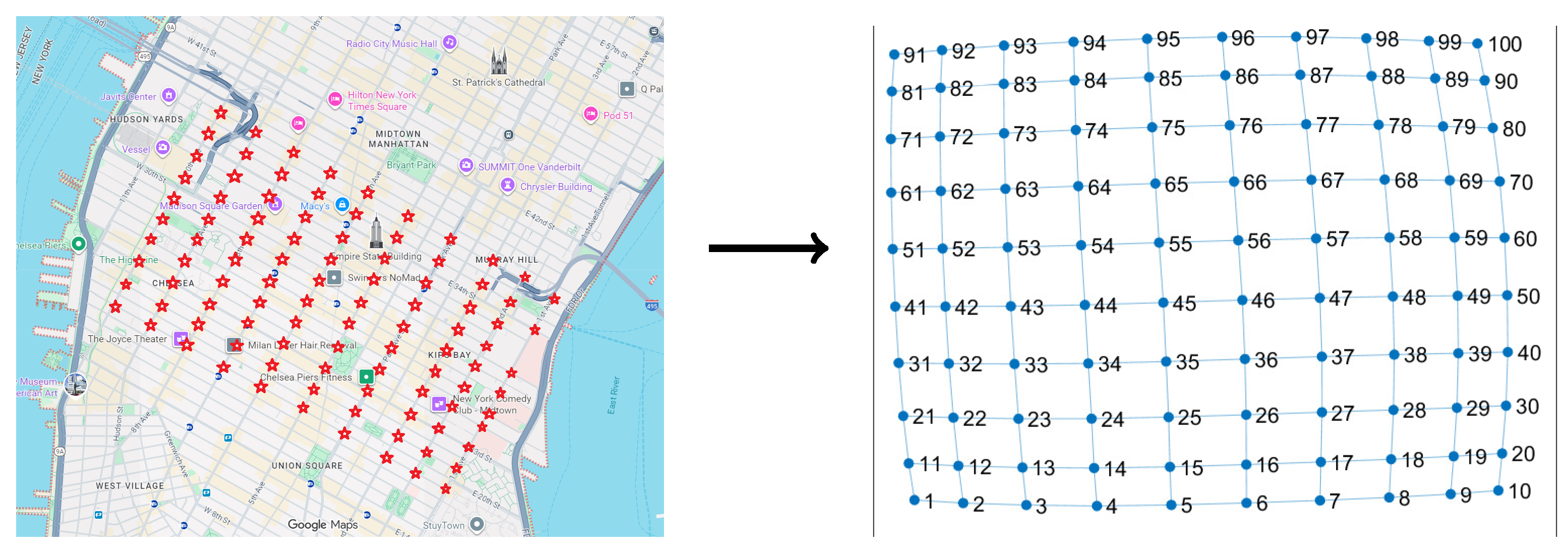
Figure 2.
Overall process flow of the proposed profit-aware EV utilisation model; Here, for PAUM-EV-M1, (C1)—(C2) stands for (8,11)—(29); for PAUM-EV-M2, (C1)—(C2) stands for (7)—(26); for PAUM-EV-M2b, (C1)—(C2) stands for (7)—(20,22)—(26,30,31)
Figure 2.
Overall process flow of the proposed profit-aware EV utilisation model; Here, for PAUM-EV-M1, (C1)—(C2) stands for (8,11)—(29); for PAUM-EV-M2, (C1)—(C2) stands for (7)—(26); for PAUM-EV-M2b, (C1)—(C2) stands for (7)—(20,22)—(26,30,31)
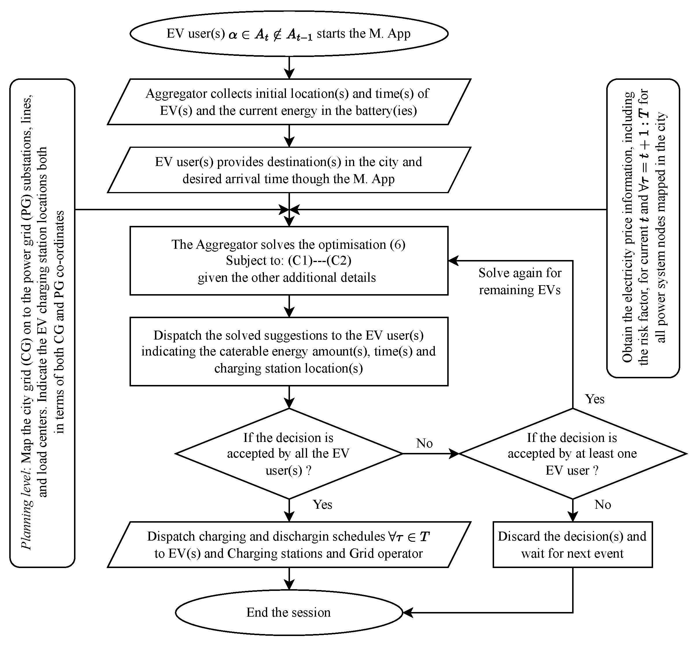
Figure 7.
(a, Left) Nodal price variations across the buses hosting EV charging stations; (b, Right) Changes made in the routes of EV to support city’s power imbalance and increase profit for EV users. Blue line indicates the original route of the EV before planning requiring charging. Green line indicates the the re-routing of the EV and selection of EVCS at minimum distance by the traditional charging algorithm without considering the profit factor. Brown line indicates the route and EVCS selected by the PAUM-EV-M1 considering all factors including the distance and the nodal prices.
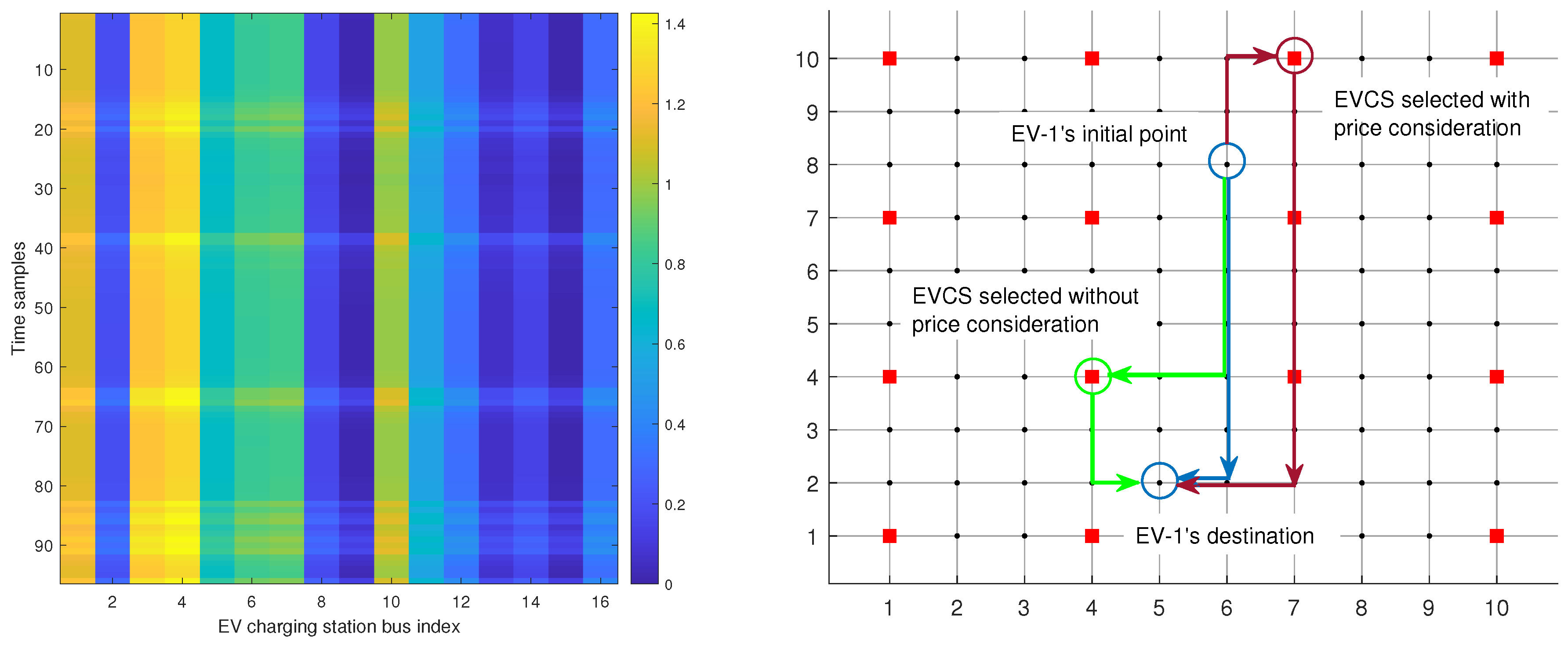
Figure 8.
Performance of traditional charging strategy (left column) and performance of PAUM-EV-M1 (right column): [Row-1 (a & b)] Total cost to EVs in $; [Row-2 (c & d)] Total distance travelled by EVs in km; [Row-3 (e & f)] Total time required to reach the destination for all EVs in min.; [Row-4 (g & h)] All 30 EVs’ battery energy levels showing charging patterns.

Figure 9.
Performance of traditional charging and discharging strategy (left column) and performance of PAUM-EV-M2 (right column): [Row-1 (a & b)] Total cost to EVs in $; [Row-2 (c & d)] Total distance travelled by EVs in km; [Row-3 (e & f)] Total time required to reach the destination for all EVs in min.; [Row-4 (g & h)] All 30 EVs’ battery energy levels showing charging and discharging patterns.
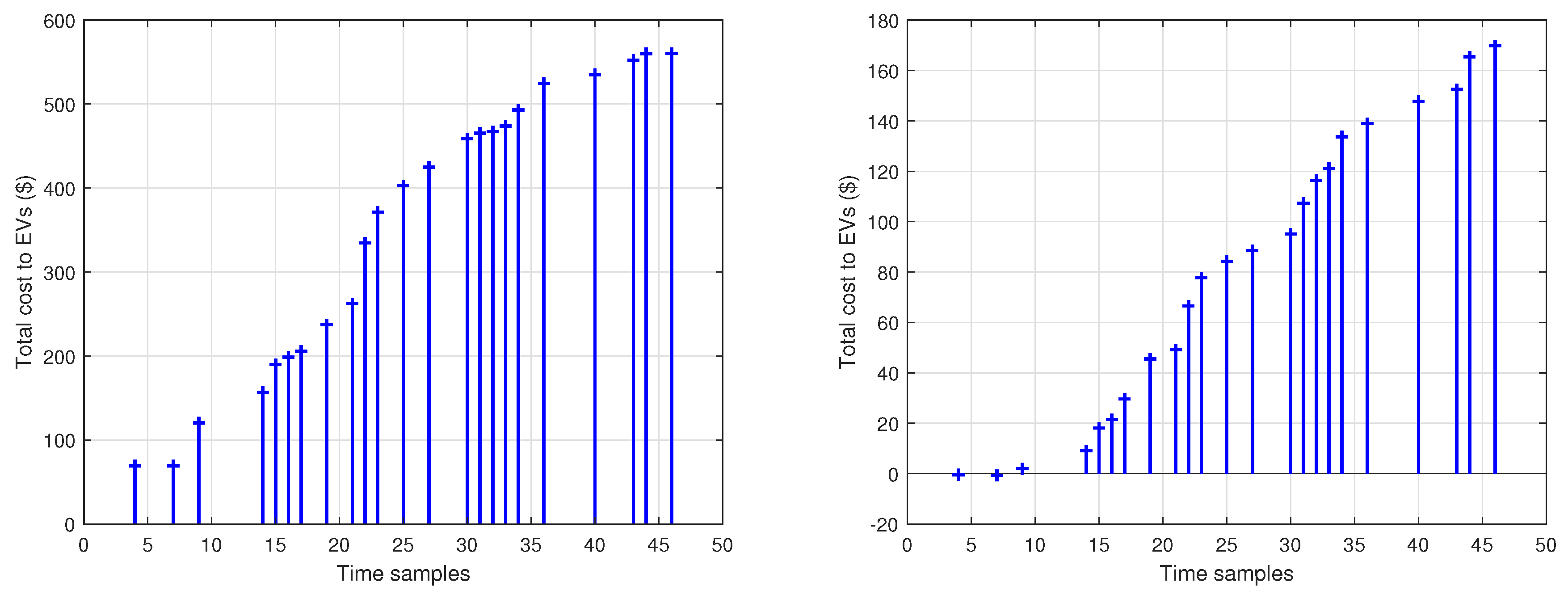
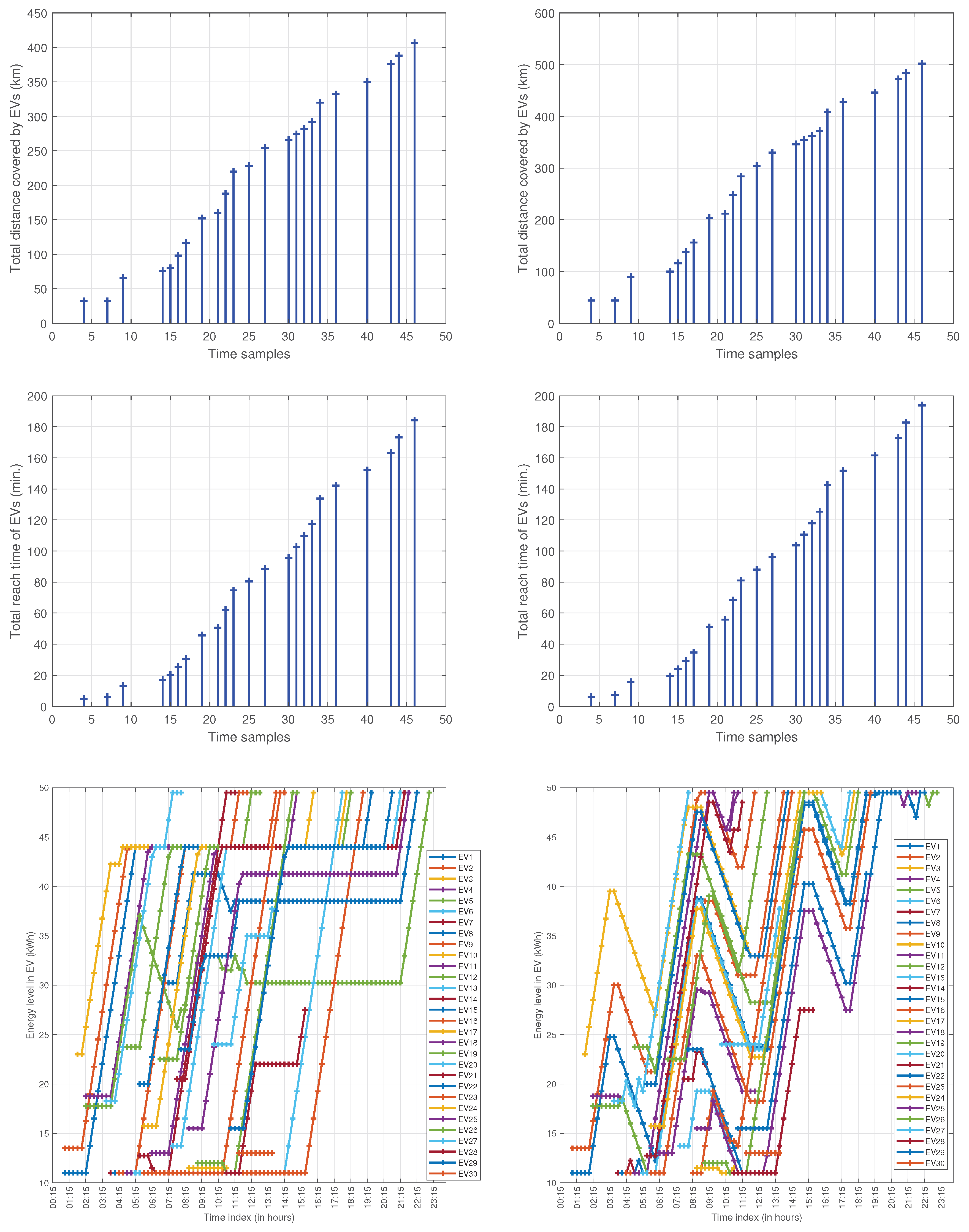

Table 1.
Impact of flexible demand management (FDM) on the aggregated non-EV loads on each bus.
| Bus no.: | 1 | 2 | 3 | 4 | 5 | 6 | 7 | 8 | 9 | 10 | 11 | 12 | 13 | 14 |
|---|---|---|---|---|---|---|---|---|---|---|---|---|---|---|
| No FDM: | 0 | 9.6 | 8.64 | 11.52 | 5.76 | 5.76 | 19.2 | 19.2 | 5.76 | 5.76 | 4.32 | 5.76 | 5.76 | 11.52 |
| FDM: | 0 | 9.3566 | 5.8518 | 9.1929 | 4.2996 | 4.4524 | 17.86 | 18.281 | 4.2345 | 4.2277 | 1.8671 | 3.3755 | 3.827 | 10.384 |
| Bus no.: | 15 | 16 | 17 | 18 | 19 | 20 | 21 | 22 | 23 | 24 | 25 | 26 | 27 | 28 |
| No FDM: | 5.76 | 5.76 | 5.76 | 8.64 | 8.64 | 8.64 | 8.64 | 8.64 | 8.64 | 40.32 | 40.32 | 5.76 | 5.76 | 5.76 |
| FDM: | 3.3253 | 4.1615 | 4.7078 | 5.823 | 6.0122 | 6.9895 | 6.7726 | 6.8789 | 8.0168 | 39.416 | 38.907 | 5.0685 | 3.2271 | 5.1757 |
| Bus no.: | 29 | 30 | 31 | 32 | 33 | |||||||||
| No FDM: | 11.52 | 19.2 | 14.4 | 20.16 | 5.76 | |||||||||
| FDM: | 10.842 | 18.688 | 14.4 | 20.16 | 5.76 |
Note: FDM stands for Flexible Demand Management.
Disclaimer/Publisher’s Note: The statements, opinions and data contained in all publications are solely those of the individual author(s) and contributor(s) and not of MDPI and/or the editor(s). MDPI and/or the editor(s) disclaim responsibility for any injury to people or property resulting from any ideas, methods, instructions or products referred to in the content. |
© 2025 by the authors. Licensee MDPI, Basel, Switzerland. This article is an open access article distributed under the terms and conditions of the Creative Commons Attribution (CC BY) license (http://creativecommons.org/licenses/by/4.0/).
Copyright: This open access article is published under a Creative Commons CC BY 4.0 license, which permit the free download, distribution, and reuse, provided that the author and preprint are cited in any reuse.


