
Submitted:
04 December 2025
Posted:
05 December 2025
You are already at the latest version
Abstract
Bridge decks are exposed to chloride ingress from de-icing salts, freeze-thaw cycling, and repeated wetting and drying, which gradually degrades the concrete over time. Many existing models treat concrete conditions as static and do not capture time-varying chloride exposure. This study develops deterioration envelopes for concrete bridge decks that predict loss of compressive strength and internal integrity by combining accelerated laboratory testing with in-situ bridge core data extracted from Delaware bridges. The model is supported by three data sources: accelerated laboratory tests, cores from in-service bridges provided by the Delaware Department of Transportation (DelDOT), and climate and asset datasets from the National Oceanic and Atmospheric Administration (NOAA) and the Federal Highway Administration's (FHWA) InfoBridge™ database. Laboratory specimens (n = 300) were reproduced based on Delaware mix designs from the 1970s and 1980s and were tested in accordance with ASTM and ACI protocols. Environmental conditioning applied wet-dry and freeze-thaw cycles at chloride contents of 0, 3, and 15 percent to replicate field exposure within a shortened test period. Measured properties included compressive strength, modulus of elasticity, resonance frequency, and chloride penetration. Results show a gradual, near-linear reduction in compressive strength and resonance frequency with increasing chloride content over 160 cycles, which corresponds to about 2 to 5 years of service exposure. Resonance frequency was the most sensitive indicator of internal damage across the tested chloride contents. By combining test results, core data, and bridge inspection history into a single durability index, the deterioration envelopes forecast long-term degradation under different chloride exposures, providing a basis for prediction that extends beyond visual inspection.
Keywords:
accelerated laboratory testing
; chloride ingress
; concrete bridge decks
; deterioration envelopes
; durability index
; freeze thaw cycling
; resonance frequency
; wet dry cycles
1. Introduction
Bridges are central components of highway and local transportation networks, providing safe passage for people and freight across rivers, wetlands, rail lines, and low-lying coastal areas [1,2]. The United States has about 617,000 bridges, and the 2021 ASCE Infrastructure Report Card noted that 42 percent of them are at least 50 years old, while about 7.5 percent are in poor or structurally deficient condition, which confirms that age related deterioration is a system level issue rather than a few isolated cases [3,4].
Among bridge components, the deck most often shows distress first, because it is directly exposed to traffic abrasion, deicing salts, freezing thaw cycles, and wetting and drying, especially in cold or marine influenced regions [5,6,7]. A primary driver of this deterioration is chloride-based deicing salts, essential for winter road safety, which significantly accelerates the deterioration of bridge decks through concrete degradation and reinforcement corrosion, leading to substantial economic costs from traffic disruptions and reconstruction. While direct data on salt application is scarce, climatic conditions can serve as exposure proxies [8,9]. This creates a critical challenge for agencies like the Delaware Department of Transportation (DelDOT), whose interstate bridge decks from the 1980s-90s are nearing the end of their typical 30-year lifespan. To optimize maintenance funding and extend service life, state agencies have developed bridge deterioration models to predict structural decline and guide proactive interventions [10]. As bridges age, repeated traffic loading and exposure to chloride laden moisture increase the need for maintenance, repair, and replacement.
With the increased use of deicing salts for vehicular safety and the threat of increased saltwater encroachment, there is a critical need to accurately predict concrete bridge deck deterioration due to chloride exposure for effective maintenance planning. For decades, research has focused on steel reinforcement as the critical component when it comes to chloride-induced damage. For example, Demich [11] investigated bridge deck deterioration caused by de-icing chemicals and observed that reinforcement in concrete bridge decks deteriorates significantly due to chloride ingress from de-icing salts, leading to corrosion and reduced structural integrity. Jia (2022) [12] analyzed the effect of reducing the cross-sectional area of reinforcing bars due to corrosion on the flexural and shear strength of typical concrete bridge decks. The authors employed ground-penetrating radars to detect corrosion probability at the top reinforcement layer; they subsequently evaluated the structural performance under both flexural and shear failure modes. The study concluded that typical levels of reinforcement corrosion were not sufficient to cause bridge deck collapse under design loading. Hájková et al. (2018) [13] present a chemo-mechanical model that links chloride ingress, corrosion initiation, cover cracking and spalling, and the resulting loss of reinforcement area in concrete structures. Applied to two existing chloride-exposed bridges, the model shows that even very small cracks can greatly shorten the predicted time to corrosion initiation, while the analyzed members still retain more than half of their original load-carrying capacity after long-term exposure. Qasim et al. [14] investigated the effect of salinity on the mechanical properties of concrete, including compressive, splitting tensile and flexural strengths. Concrete specimens cured in NaCl solutions with salt contents between 0% and 5% by weight of water showed an overall reduction in 28-day strength with increasing salinity; for example, the 28-day cylinder compressive strength decreased from 30.0 MPa at 0% salt to 26.1 MPa at 5% salt. The authors attributed these reductions to the damaging action of dissolved salts and associated sulfate attack on the hardened cement paste. Penttala [15] investigated concrete exposed to freeze–thaw in water and in a 3% NaCl solution and found that the water–cement ratio and air content largely control both surface scaling and internal damage. Concretes with lower water–cement ratios and sufficient air entrainment showed better resistance, while saline freeze–thaw at low water–binder ratios led to more internal damage and required higher air contents to limit it
Despite significant research on reinforcement bar corrosion-induced deterioration, many transportation agencies have increasingly adopted corrosion-resistant strategies, such as epoxy-coated reinforcement, reducing its role as the primary cause of deterioration [16]. While this effectively delays steel deterioration [17], it shifts the primary mode of failure and the concrete itself then becomes the critical component governing deck service life. This shift creates a fundamental gap in existing predictive models, since the traditional models [17,18] were developed and calibrated largely consider corrosion-based deterioration, as uncoated reinforcement will lead to spalling and cracking of concrete decks. They are therefore inadequate for predicting the long-term degradation of the concrete material, which is now the controlling factor in the service life of modern bridge decks. This shift means that future predictive models should place more weight on long term concrete material degradation and should define deterioration envelopes that include newer preservation practices and materials
While bridge deterioration models are important for optimizing maintenance planning and for allocating limited funds [18], models that rely only on historical inspection data have a built-in limitation. In Delaware, for example, DelDOT’s model uses the National Bridge Inventory ratings to learn past deterioration patterns and to project future condition, which works well when the bridge stock and materials stay similar over time. Most of these datasets, however, reflect decks with uncoated reinforcement, so the forecast is driven mainly by corrosion induced spalling and cracking [17]. Once epoxy coated reinforcement and other anticorrosion techniques became common in Delaware bridge construction in the 1970s, the steel component of deterioration was delayed [19]. In that case, the concrete itself can become the governing limit on deck service life, not the reinforcement. This shift means that future predictive models should place more weight on long term concrete material degradation and should define deterioration envelopes that include newer preservation practices and materials.
The objective of this research is to evaluate the impact of salinity exposure on cementitious materials in terms of accelerated and projected long term structural performance and durability, and to develop deterioration envelopes for predicting concrete bridge deck deterioration due to chloride exposure. Accelerated laboratory tests in an environmental chamber at specified chloride concentrations and temperatures are combined with deterioration trends and existing condition state data to generate long term curves for chloride induced damage. Bridge deck cores taken from structures older than 50 years are used as a baseline for comparison and for validating the experimentally derived trends. The novelty of this work lies in the combined use of accelerated environmental chamber testing, multi parameter material characterization, and in-situ bridge deck cores to derive deterioration envelopes that are calibrated against field performance in high salinity conditions. The study examines the influence of cyclic wet/dry exposure and freeze/thaw cycles on the mechanical properties and durability of concrete, with a focus on the role of salt concentration in promoting microstructural degradation and loss of strength. Material degradation is quantified by measuring compressive strength, modulus of elasticity, Poisson’s ratio, and chloride penetration. The resulting predictive deterioration envelopes provide a clearer view of deterioration progression in concrete infrastructure and the resilience of concrete in harsh exposure. In the long term, the findings are intended to inform the degradation models used by the Delaware Department of Transportation (DelDOT), with particular focus on the performance of concrete bridge decks that utilize corrosion resistant steel reinforcement in high salinity environments, and to support preservation strategies and long-term durability assessments of critical transportation infrastructure.
2. Materials and Methods
2.1. Materials
The materials used in this study were selected in accordance with the State of Delaware State Highway Department Standard Specifications from the 1970, 1974, and 1985 editions. The selection of these materials ensured consistency with historical construction practices relevant to Delaware’s bridge infrastructure. Table 1 presents the physical properties of the cement, fine aggregate, and coarse aggregate used in the mix design, sourced to reflect a modern equivalent of the cement components used during the era under investigation. Additionally, the table includes the batching weights for a cubic yard of concrete, along with a scaled version for a cubic foot of concrete, which served as the basis for batching and casting the concrete specimens. To ensure an accurate water-to-cement ratio (w/c), the aggregated water content was determined in accordance with ASTM C70 [20]. The finalized w/c ratio is provided in the table below. All material testing followed ASTM Standards.
2.1.1. Cement
Ordinary Portland Cement (Type I) was utilized in this study, conforming to ASTM C150 specifications. The cement was sourced from Keystone Cement Company to maintain consistency in material properties across all experimental procedures. The parameters of the cement used in the test were shown in Table 1.
2.1.2. Aggregates
The fine aggregate used in this study consisted of C33 sand with a rough surface texture, selected based on its compliance with ASTM C33 [21]standards. The physical properties of the fine aggregate were determined in accordance with the relevant testing protocols and are detailed in a subsequent section. The coarse aggregate employed in this study was C57 stone with a nominal size of 19 mm, in accordance with ASTM C57 specifications. The mix design properties for the coarse aggregate are presented in Table 1.
3.1.3. Admixtures
The Delaware Department of Transportation (DelDOT) Standard Specifications from 1970, 1974, and 1985 editions did not specify the use of admixtures. However, air content requirements were explicitly defined. To ensure compliance with these specifications and maintain the appropriate air content in the replication mix, an air-entraining admixture was incorporated. This addition facilitated the proper entrainment of air voids, which is critical for enhancing the durability and freeze-thaw resistance of the concrete.
2.2. Experimental Methodology
2.2.1. Concrete Mix Design
The concrete mix design for the laboratory samples was developed as a replication mix based on historical standards obtained from DelDOT practices. While this mix was selected to represent the typical concrete used in Delaware bridge deck construction during the 1970s and 1980s, it does not constitute an exact reproduction of the materials and proportions used at the time. Variability in contractor practices, material sourcing, and project-specific requirements likely led to differences in the concrete mixes used across various bridge decks. The laboratory mix employed in this study represents one potential formulation that aligns with historical standards from that period and serves as a basis for further investigation.
2.2.2. Sample Preparation
Given the large number of laboratory samples required to develop a robust dataset, the concrete components were batched beforehand to a volume totaling 0.07 CBM to facilitate proper mixing within the concrete mixer. The aggregates, cement, admixtures, and water were measured in 0.0189 m³ buckets and sealed to prevent any changes in moisture content between the weighing and mixing stages. A Marshallton drum mixer shown in Figure 1 was used for the casting process, as its mixing mechanism closely replicates the method employed by concrete trucks in the field when casting bridge decks. This ensured consistency in the mixing process and alignment with real-world construction practices.
The mixing process followed a structured sequence to ensure proper hydration, dispersion, and homogeneity of the concrete mix: The entire mixing process was completed in under 20 minutes per batch to maintain consistency and workability.
2.2.4. Fresh Concrete Properties
The workability assessment of the fresh concrete mixtures was conducted by measuring the slump height following the procedures outlined in ASTM C143 [22]. The test involved using a standard slump cone with an upper diameter of 100 mm, a lower diameter of 200 mm, and a height of 300 mm. The test was repeated three times for each mixture to ensure statistical reliability.
The fresh unit weight of the concrete was determined using an air content chamber pot, which has a standardized volume of 0.00707 CBM. The measured fresh unit weight ranged from 65.3 to 66.22 kg/m3, aligning with the expected values for the designed mix. The air content of the fresh concrete mixtures was determined using the pressure method following the procedures outlined in ASTM C231 [23]. To ensure accuracy and repeatability, the test was performed three times for each mixture. The measured air content ranged from 5.5% to 7%, which was within the target range consistent with historical concrete mix practices.
2.2.5. Conditioning of Samples
To replicate field deterioration mechanisms, two accelerated conditioning regimes were employed: wet-dry and freeze-thaw cycling. Specific salinity concentrations and exposure durations were selected to mirror aggressive service environments characterized by heavy deicing salt applications. These controlled parameters adhere to established industry standards; they provide a rigorous baseline for correlating laboratory outcomes with the in-situ performance of extracted bridge cores. The concrete samples were subjected to three distinct conditioning regimes to represent different environmental exposures:
Wet-Dry Cycling samples were submerged in saline solutions (0%, 3%, and 15% by weight) for 12–14 hours and air-dried under fans for the remainder of the 24-hour. This process simulates cyclical moisture fluctuations commonly experienced in bridge decks and other exposed concrete structures. The duration of each phase ensured full specimen saturation and drying. A cumulative 154 cycles were conducted to emulate the long-term environmental impacts of moisture exposure under high chloride concentrations.
Freeze-Thaw Cycling samples were subjected to repeated freezing and thawing cycles replicating seasonal temperature variations. This process followed ASTM C666 [24] procedures, which consisted of 12–14 hours at sub-zero temperatures (-25°C) to simulate frost exposure in an environmental chamber (Figure 2). Following freezing, the samples were soaked in the respective water baths (0%, 3%, or 15% salt solutions) to thaw for the remainder of the 24-hour cycle.
A total of 140 cycles were performed to model the synergistic impact of both moisture exposure and freezing temperatures on the deterioration of concrete. Such cycles simulate one of the most severe environmental conditions for bridge decks, in which water penetrates the concrete, freezes, and expands, causing internal cracking, surface scaling, and long-term structural damage. For a control condition, the samples were stored under standard conditions in a fog room maintained at 26.7°C and 90% relative humidity to serve as a baseline for comparison with the accelerated aging conditions.
Selected chloride concentrations simulate two distinct salinity sources typical of concrete exposure environments. The 3% solution approximates seawater salinity: the 15% solution replicates brine concentrations utilized in road deicing. Although DelDOT standard brine solutions range from 20% to 25% salinity, effective concentrations on the road surface decrease due to mixing with snow and ice. Consequently, the 15% concentration was determined to better represent realistic field exposure. This conditioning regime was repeated for the duration of the test period, ensuring that the environmental stresses on the samples were consistent with real-world exposure conditions. Regular testing intervals of 14 cycles were implemented to monitor changes in material properties over time. A total of 11 sets of cycles were conducted for the wet-dry cycling, and 10 sets of cycles were conducted for the freeze-thaw testing.
2.3. Concrete Core Testing of Delaware Bridges
To correlate laboratory-observed deterioration with real-world conditions, in-situ bridge cores were obtained for testing by the DelDOT. To minimize the risk of contamination during transport to the laboratory, the cores were sealed in plastic bags, as illustrated in Figure 3(a). A total of 22 cores were extracted from two bridge locations: the James Street Bridge in Newport and the I-495 –800-series (based on naming convention) of bridges owned by DelDOT. The compressive strength results from these cores were compared to data from deck cores previously tested by DelDOT from the same bridges, as well as a broader dataset of bridge cores.
Since the cores were extracted from active bridges, they required preparation before testing. This process involved trimming them with a concrete circular saw equipped with a diamond blade to remove damaged ends and achieve parallel surfaces, in accordance with ASTM C42. The cores were trimmed to their maximum savable length to eliminate damage from the extraction process. Because the trimming process used water, the cores were allowed to surface dry before capping, as shown in Figure 3 (b-c). For cores with slightly damaged ends or to minimize excessive length loss, a sulfur capping compound was used to create parallel loading surfaces following ASTM C617. The capped specimens were cured for one hour before testing, and a second set of photographs was taken for documentation. The concrete cylinders were loaded into the Humboldt compression machine as seen in Figure 3 (d) and carefully centered on the platens to ensure uniform loading. Compressive testing was conducted at a controlled loading rate of 99.79 kg/sec, in accordance with ASTM C39 – Standard Test Method for Compressive Strength of Cylindrical Concrete Specimens. The test continued until the cylinders failed, maintaining a load approximately 20% below the maximum applied load to ensure consistent failure conditions.
2.3.1. Mechanical Testing Procedures
The Mechanical Testing portion of the study is detailed in this section and includes the physical testing procedures used to evaluate material performance. These tests consist of Resonance Frequency Testing, Compressive Strength, Modulus of Elasticity, and Poisson’s Ratio measurements.
- a)
- Resonance Frequency Testing
To monitor the progression of deterioration in the concrete samples, a non-destructive evaluation method was used. The dynamic modulus of elasticity was assessed by measuring the longitudinal mode of resonance frequency in accordance with ASTM C215 [25], Standard Test Method for Fundamental Transverse, Longitudinal, and Torsional Frequencies of Concrete Specimens. This method was used to quantify material degradation in concrete subjected to wet–dry cycling and freeze–thaw cycling in water baths with salt concentrations of 0%, 3%, and 15% by weight. Testing was performed at 14-cycle intervals to track changes in the mechanical properties of the concrete overtime. Before each measurement, samples were allowed to dry after completion of the fourteenth cycle to keep the test setup consistent. The equipment, shown in Figure 4(a), included a resonance testing gauge with an accelerometer attached to one end of the concrete specimen using acoustic grease to ensure good contact and signal transfer. A schematic of the resonance testing procedure is given in Figure 4(b). During testing, the concrete specimen was tapped with a small hammer to induce vibration at its natural frequency.
The accelerometer captured the resulting motion as a voltage signal, which was processed by a data acquisition program to convert the signal into a frequency measurement in hertz. These measurements were recorded at each interval to build a history of deterioration for every specimen before destructive testing. This approach made it possible to relate changes in resonance frequency to changes in the physical properties of the concrete, and to study how environmental exposure, cyclic loading, and salt concentration influence the structural integrity of the material over time.
- b) Compression Testing
To quantify the physical deterioration of the laboratory samples during cyclic exposure, the compressive strength of concrete was evaluated in accordance with ASTM C39 (Standard Test Method for Compressive Strength of Cylindrical Concrete Specimens). This test assessed the effects of moisture fluctuations, freezing, and varying salt concentrations on the mechanical integrity of the concrete. Specimens from each test group were removed every 14 cycles for compressive strength testing. In accordance with ASTM C39 [27], three specimens were tested at each interval. Neoprene pads in steel retaining collars were used to provide uniform loading surfaces and consistent testing conditions. The concrete cylinders were then loaded into the Humboldt compression machine and centered on the loading platens for proper alignment. Compressive loading was applied at a controlled rate of 99.79 kg/sec, as specified by the standard, and continued until cylinder failure while maintaining the load approximately 20 percent below the maximum applied load to avoid premature unloading. After each test, photographs of the fractured specimens were taken for documentation, as shown in Figure 5. The maximum compressive strength of each cylinder was recorded to measure progressive deterioration due to cyclic environmental exposure. Each labeled specimen was then returned to its sealed plastic bag for subsequent chloride testing.
- c) Modulus of Elasticity Testing
The static modulus of elasticity and Poisson’s ratio of conditioned concrete cylinders were measured in accordance with ASTM C469 (Standard Test Method for Static Modulus of Elasticity and Poisson’s Ratio of Concrete in Compression). The test assessed the stiffness and strain response of specimens subjected to wet dry cycling and freeze thaw cycling. The recorded data included the static modulus of elasticity, which quantifies stiffness after cyclic exposure, and Poisson’s ratio, which describes the relationship between lateral and axial strain under compressive stress. A stress–strain curve was generated for each specimen to describe behavior after environmental cycling. During testing, each specimen was centered in the apparatus both laterally and vertically to obtain consistent measurements, as shown in Figure 6. Two Linear Variable Differential Transformers (LVDTs) recorded radial and axial deformation, enabling calculation of stress and strain throughout the test. Testing used a Humboldt compression machine with a compressometer/extensometer for automated loading and data collection. The maximum load was limited to 40 percent of the expected compressive strength of each sample to avoid damage to the rings and LVDTs. Following the completion of modulus testing, the specimens were subjected to compressive strength testing, as described previously. After testing, each labeled specimen was carefully returned to its sealed plastic bag for subsequent chloride testing, ensuring proper sample preservation for further chemical analysis, as illustrated in Figure 5 (b).
2.3.2. Resistivity Testing Procedure
Water soluble chloride content was measured to relate salinity to the resistivity of each laboratory sample, following ASTM C1218 with minor adjustments for the large number of specimens. Concrete cores were first reduced to powder using a hand operated rock crusher, as shown in Figure 7(a). The crushed material was sieved through a No. 20 soil sieve (850 µm); the passing fraction was collected, sealed in clean plastic bags, and thoroughly mixed to obtain a homogeneous sample. The crusher and sieve were cleaned after each batch to avoid cross contamination.
Powdered samples were tested in a clean laboratory. For each cylinder, three subsamples of 5.00 ± 0.01 g were weighed on clean weighing paper, as shown in Figure 7(b). Each subsample was placed in a container with 40 mL of deionized water and left for 24 h to dissolve water soluble chlorides, then remixed and allowed to settle for 30 min. A handheld salinity meter, Figure 7(c), was used to measure chloride concentration in the supernatant. These measurements were used to judge whether damage in the specimens was governed mainly by the physical effects of freeze-thaw and wet dry cycling or by chemical attack associated with elevated chloride content in the concrete.
3. Results
3.1. Physical Results
3.1.1. Resonance Frequency
Resonance frequency tests were carried out to track the internal condition of the concrete specimens during the entire period of the laboratory tests for durability. The test enabled continuous observation of material deterioration prior to the actual application of the compressive strength tests on the specimens. Figure 8 demonstrates the temporal behavior of individual resonance frequencies for specimens subjected to wet-dry exposure at three salinity levels. This monitoring approach allows for a more refined understanding of how wet-dry exposure affects material behavior.
The overall trends for the salinity of soaking solutions show that the presence of chlorides affects deterioration. Figure 9 presents the temporal behavior of resonance frequency for specimens exposed to freeze-thaw cycling. This exposure mechanism has the most severe overall downward trend in resonance frequency, showing that freeze-thaw action produces the greatest reduction in dynamic stiffness among the tested exposure categories. As in the wet-dry series, the trends for different salinity levels indicate that the presence of chlorides affects the deterioration process.
The resonance frequency response of the control specimens is shown in Figure 10. In contrast to the wet-dry and freeze-thaw series, the control specimens exhibit an increase in resonance frequency over time. This behavior reflects the absence of aggressive environmental exposure and provides a reference for interpreting the downward trends observed in the cycled specimens. These trends are used in subsequent analysis to predict the overall long-term deterioration that bridge decks can potentially face.
As the resonance testing had the largest number of samples in its testing series over the course of the deterioration cycling, the trends were used to forecast the loss in strength over time in the sections discussed further.
3.2.2. Compressive strength
The compressive strength test was conducted to evaluate the load-bearing capacity of the concrete samples as they were subjected to simulated deterioration regimes. The strength development in each exposure group is shown in Figure 11 (a–c), illustrating the effect of wet-dry cycling, freeze-thaw exposure, and chloride saturation on the rate and magnitude of compressive strength loss. These trends are used to assess how quickly the material deteriorates under accelerated aging and to compare the relative severity of each exposure regime.
Although these results provide useful insight, the compressive strengths measured in this study exhibit considerable scatter. As shown in the 50-year concrete strength study reported by [28], the strength gain of concrete over time follows a logarithmic curve, and early-age data lie in the nonlinear part of this relationship. Because the present testing was performed at an early stage in the concrete life cycle, the variability in strength was too high to isolate the effects of chloride content based on compressive strength alone.
3.2.3. Modulus of Elasticity
The modulus of elasticity test was conducted to examine the stiffness and deformation response of the concrete specimens under load. Figure 12 (a–c) presents the temporal development of the modulus for specimens exposed to wet-dry cycling and freeze-thaw cycling at three salinity levels, 0, 3, and 15 percent, with a control series included for comparison.
Across all exposure regimes and salinity levels, the measured modules remain within a relatively narrow band and exhibits only a modest overall reduction as the number of cycles increases. Changes in stiffness are therefore small compared with the variations observed in the other material properties, and no strong, systematic separation between the different salinity levels is evident. This variability indicates that additional investigation is needed before modulus degradation can be used reliably as a parameter in the deterioration model. Increasing the number of cycles or extending the exposure duration in future tests may generate larger stiffness losses and clearer trends, which would improve the ability to use modulus degradation in long term deterioration assessment.
3.2.4. Poisson’s Ratio
Poisson’s ratio was measured to quantify the lateral strain response of the concrete specimens under axial loading. It is defined as the ratio of transverse strain to axial strain and provides an indicator of changes in the internal microstructure due to environmental exposure. Figure 13 (a–c) shows the evolution of Poisson’s ratio with cycle number for the different exposure regimes and salinity levels, and these results are used as supporting information alongside modulus of elasticity and compressive strength to interpret the progression of deterioration. Due to a data acquisition error, Poisson’s ratio values at 112 cycles are missing in Figure 13 (a) and were excluded from interpretation.
3.2.5. Compressive and Resonance Frequency Comparison
Using both test methods together provides complementary destructive and non-destructive evaluations of material performance over the duration of the laboratory program. The compressive strength results quantify the reduction in load carrying capacity as deterioration progresses and indicate how the concrete resists the applied loads. In parallel, resonance frequency measurements offer a non-destructive means to detect internal changes in stiffness and microstructural condition before visible cracking or loss of load carrying capacity occurs. Comparison of these two datasets relates internal degradation, reflected by changes in resonance frequency, to the corresponding loss in compressive strength. The combined use of resonance frequency and compressive strength provides a clearer picture of damage development in the concrete and improves the ability to identify early signs of performance loss, demonstrating the benefit of incorporating multiple performance measures in durability testing.
3.3. Chemical Results
The chemical results focus on the water-soluble chloride content of the concrete samples. The measured chloride concentrations are used to interpret the deterioration observed in the durability cycles and to assess how chloride penetration relates to reductions in compressive strength, modulus of elasticity, and resonance frequency. These findings support the broader goal of distinguishing mechanical deterioration from chloride-driven degradation in bridge decks. The laboratory chloride profiles are also compared with in situ bridge core data to check the consistency of the observed trends.
As detailed in section 2.3.2, water soluble chloride content was determined on more than 250 specimens, with three replicate measurements per specimen, yielding over 750 individual test results. After completion of the exposure cycles, the concrete was powdered and analyzed for water soluble chlorides, representing the fraction of chlorides available to participate in chemical degradation. For each exposure group, multiple specimens were combined to obtain a representative average chloride content that reflects variations in mixture composition, porosity, and penetration depth. Figure 14 (a–c) summarizes the average chloride contents for wet dry, freeze-thaw, and control specimens at the different saline solution concentrations. The results indicate that differences between the two accelerated deterioration regimes are small, and that internal chloride accumulation is governed primarily by the concentration of the soaking solution.
4. Case study: Delaware Bridges
4.1. Selected Bridge Locations
To validate the laboratory findings, bridge deck cores from selected Delaware bridges were evaluated alongside the laboratory-cast specimens and compared with data supplied by the Delaware Department of Transportation (DelDOT) and its consultant. This case study presents an in-situ investigation of bridge deck deterioration based on core samples drilled from Interstate 495 (I-495) in Wilmington, Delaware, as shown in Figure 15.
The selection of I-495 was based on recent evaluations and reports that document deck condition and provide information on environmental exposure, traffic loading, and material performance. The bridge cores analyzed in this study were obtained as part of a DelDOT investigation carried out by one of DelDOT’s contractors, and the associated data were provided to support the present work.
Delaware provides a well-documented example of effective bridge management, with a clear focus on infrastructure preservation through targeted resource allocation and proactive maintenance. The DelDOT reports an overall bridge condition rating of about 98 percent. This high network rating reflects sustained attention to structural integrity and serviceability. At the same time, all bridges undergo long term deterioration, and there is a need to better quantify these processes; the present study contributes to that goal. As shown in Figure 16, most Delaware bridges fall within the “Good” condition rating, and relatively few are classified as Poor. While this outcome is favorable for network performance, it also limits the availability of bridge cores representing advanced deterioration, which makes it challenging to assemble a broad field dataset spanning a wide range of damage levels.
By studying these bridge cores, the present case study links laboratory observations with field performance and reduces the gap between controlled tests and concrete bridge decks exposed to real environments. Although the exposure histories of the decks were not controlled, cores from bridges of different ages provide useful information on how deterioration develops with time and support decisions on maintenance and rehabilitation. Cores are used to evaluate material performance, identify degradation mechanisms such as cracking, delamination, and corrosion, and supply data for refining predictive models of bridge deck life.
Most of the bridge decks from which cores were extracted are still rated “Good,” which reflects Delaware’s preventive bridge management but limits the range of observed deterioration states. Heavily degraded decks are rare, so there are few cores from advanced damage levels; nonetheless, the available cores document early deterioration and long-term aging in maintained decks. Within this context, the study also examines how reinforcement protection and repair strategies, such as epoxy coated bars, corrosion inhibitors, and overlays, influence deck ratings over time on the I-495 viaduct and how rating improvements and their duration relate to specific maintenance actions.
4.2. Bridge Deck Cores
To gain first-hand information on material performance and degradation mechanisms after a full in-service life, physical testing was conducted on core samples of bridge deck concrete gathered from 31 bridges in Wilmington, Delaware. The core samples provide critical information on the durability of concrete, offering in situ confirmation of laboratory findings on compressive strength, salinity content, and petrographic features.
4.2.1. Core Sample Testing and Analysis
The laboratory tests conducted on the samples yielded comprehensive reports on the structural condition, material composition, and degradation patterns that gave essential information for the bridge deck effectiveness assessment. To analyze the properties of materials, standard testing was conducted. Compressive strength testing established load-bearing capacity, a key indicator of structural integrity. Salinity testing quantified chloride penetration of deicing salts, which accelerates corrosion of reinforcement. Petrographic analysis provided a microscopic assessment of aggregate composition, cracking patterns, and cement matrix structure. Although the petrographic analysis was not a key factor in the analysis of the study, it did provide some reasoning for several samples that were outliers in the reports.
The study also juxtaposed the relationship between material performance and the age of bridges to determine if older bridges exhibit more deterioration or if better construction materials and maintenance strategies have extended service life. In Figure 17, the ages of the bridges examined compares patterns of deterioration during different construction periods. Correlating core sample performance with the age of bridges, this study informs long-term material development and directs bridge preservation practice for the future.
4.2.2. Compressive Testing of Bridge Cores and Lab Specimens
Compressive strength measurement is a vital component of bridge deck assessment, delivering valuable information regarding the load-carrying capacity and structural integrity of concrete elements. In this research, the compressive stress of the bridge decks in question was derived from the average core sample values of the chosen bridges. For some of the core samples, the specified length-to-diameter (L/D) ratio requirement was not achieved due to several factors such as deck depth, and therefore, the application of correction factors was required to facilitate proper strength calculations. The corrected bridge deck stresses are displayed in Figure 18, showing the range of values that even the same deck can have.
Bridge deck core samples’ compressive strength testing was in line with ASTM C42/C42M [29] standards that recommend 2:1 length-to-diameter (L/D) ratio for accuracy. The ratio ensures test results reflect in situ concrete strength because variations in core dimensions may affect measurements. Some of the cores extracted were less than the preferred L/D ratio, and corrections were applied. The shorter cores would show artificially higher strengths due to reduced lateral expansion effects. To correct this, ASTM-recommended equations were applied to normalize compressive strength values based on actual L/D ratios for the sake of uniformity in samples. Following the application of correction factors, the corrected compressive strength values gave a good indication of in situ material properties. Standardizing this information allows for accurate comparisons between bridges and their deterioration trends, facilitating accurate structural assessments, and long-term durability analysis.
To make a wider comparison of compressive strength among various bridge decks, a study of the age of the core samples was conducted to determine trends in material behavior with age. Because the strength of concrete can deteriorate from exposure to the environment, cyclic loading, and chemical corrosion, placing the cores in specific age groups enables a clearer determination of the performance of aging bridge decks. The bridge core samples were categorized into age groups to examine how compressive strength varies over time as shown in Figure 19.
4.2.3. Chloride Measurements of Bridge Decks
In addition to compressive strength, the chloride content of the bridge deck cores was also measured, recognizing it as a significant parameter affecting reinforcement corrosion and long-term durability. Chloride-induced corrosion is among the most critical mechanisms of degradation of concrete bridge decks, especially in areas that receive deicing salts in winter [30]. Chloride penetration variability in bridge decks of varying ages, exposure conditions, and health and maintenance histories is investigated in this research. Figure 20 shows Chloride Content by Bridge Age provides a breakdown of chloride concentration levels across different bridge decks. Older bridges are more likely to have accumulated higher chloride concentrations due to prolonged exposure. Bridges in high-traffic areas or locations with heavy deicing salt usage tend to exhibit greater chloride intrusion. Bridges that received protective treatments (e.g., waterproofing membranes, sealants, or overlays) show lower chloride penetration compared to untreated decks.
This categorization allows for a comparative analysis of how high chloride concentrations affect concrete deterioration beyond just reinforcement corrosion. The traditional perspective views steel reinforcement as the primary limiting factor in bridge deck degradation, but this study aims to determine the extent to which chloride-induced deterioration affects the concrete matrix itself, even when reinforcement is protected. A common premise in bridge deterioration modeling is that bridge deck ratings decline over time due to progressive material deterioration, environmental effects, and traffic loading. However, a review of historical bridge deck ratings indicates that rating increases have occurred for some bridges at some time during their life-cycle. Since bridge conditions would naturally decrease without intervention, any NBI rating increase observed suggests that maintenance interventions, e.g., patching or replacement of wearing surface, occurred.
Bridge deck ratings decline with age due to material deterioration, environmental exposure, and traffic loading. Improvements in ratings are realized through maintenance operations, principally resurfacing rather than total deck replacements, which are costly and infrequent. Resurfacing enhances surface conditions but not the underlying structure, thus ratings are improved temporarily, and deck life is extended. Tracking these fluctuations provides insight into resurfacing as a maintenance practice and its impact on long-term bridge performance. Along with individual rating change, the study analyzes overall trends in deterioration to compute average decline rates across numerous bridges Figure yields three significant findings: (1) bridge decks undergo a natural deterioration trend due to wear and environmental stress, (2) there is a short-term beneficial effect of resurfacing on ratings, and (3) deterioration renews after maintenance, providing information on the effectiveness of resurfacing and optimum frequency of intervention. These findings support data-driven bridge maintenance planning, with an emphasis on the importance of timely resurfacing and its limitations in addressing more severe structural deterioration.
5. Analysis and Discussion
The analysis is organized into four primary sections, which help inform the deterioration envelope: 1) Environmental Condition Trends, 2) Experimental Trends, 3) Predictive Models, and the 4) Durability Index. Each section builds upon the results to progressively connect short-term laboratory findings with long-term deterioration behavior.
5.1. Environmental Condition Trends
This section examines the environmental factors causing degradation of concrete bridge decks, such as chloride exposure, freeze-thaw cycling, and wet-dry exposure. These exposures were simulated in laboratory testing to model real exposure conditions prevalent in Delaware and similar climates. The resulting information illuminates the effect of environmental stressors on the type and rate of degradation, forming the basis for evaluating long-term bridge deck performance.
Freeze-Thaw Predictions
The trends used for freeze-thaw cycle predictions were derived from historical weather, obtained from the NOAA weather station based in Wilmington, Delaware. An empirical relationship, represented by Equation 1, was established using this dataset and subsequently plotted against the freeze-thaw cycle counts reported in InfoBridge™, as shown in Figure 21. The resulting correlation was used to estimate annual freeze-thaw frequencies, which were then incorporated into the deterioration modeling presented later in this analysis. The number of freeze thaw cycles since construction is given by:
(1)
(2)
Where: ̶ Number of Freeze-Thaw cycles since construction
T - Years since construction
Tc - Current year
Ti - Year of construction
This equation was derived from the linear trend as shown in Figure 22. The equation presented in the figure was integrated over the interval from 0 to T (where T represents the number of years since construction) to derive an empirical relationship linking the area's climate data with the structure's age.
Snow Day Predictions
Snow day predictions were developed using historical weather data presented in Figure 23, obtained from InfoBridge™ for the bridges located along the I-495 viaduct in Wilmington, Delaware. An empirical relationship, represented by Equation 3, was derived from this dataset, and the resulting correlation was used to estimate the frequency of annual snow days. These estimates were subsequently incorporated into the deterioration modeling presented later in this analysis. Snow day frequency served as a key variable in estimating long-term chloride accumulation, as deicing salt application during snow events represents a primary source of chloride ingress in bridge decks. Number of Snow Fall Days Since Construction is given by:
(3)
(4)
Where:
NSD Number of Snow Days since construction
T Years Since Construction
TC Current Year
Ti Year of Construction
This equation was derived from the linear trend as shown in Figure 22. The equation presented in the figure was integrated over the interval from 0 to T (where T represents the number of years since construction) to derive an empirical relationship linking the area's climate data with the structure's age.
5.1.3. Wet-Dry Cycles Predictions
Wet-dry cycle predictions were developed using historical climate data presented in Figure 22, sourced from InfoBridge™ regional precipitation records relevant to the I-495 Viaduct in Wilmington, Delaware. An empirical relationship, expressed as Equation 5, was established to estimate the frequency of wet-dry cycling based on precipitation patterns and drying intervals. This correlation was used to determine annual wet-dry cycle counts, which were then integrated into the deterioration modeling presented later in this analysis. The frequency of wet-dry cycles plays a critical role in the transport of chlorides into concrete and the progressive breakdown of material integrity over time. Number of wet-dry cycles since construction is given as:
(5)
Where:
T Years Since Construction
NWDCycles Number of Wet-Dry Cycles since construction
5.2. Experimental Trends
This section presents the trends observed from accelerated laboratory testing of concrete specimens. Key physical and mechanical properties, including compressive strength, modulus of elasticity, resonance frequency, and chloride penetration, were monitored over time. The data highlights the material’s degradation behavior under different environmental conditions and helps establish baseline patterns necessary for predictive modeling.
Resonance Frequency Trends
As the resonance frequency data represented the most extensive dataset collected during the experimental phase of this study, its trends were identified as the most significant and consistent indicators of long-term strength loss due to environmental cycling. As shown in Figure 24, the average resonance frequency for each environmental condition has been plotted to illustrate the overall trend in material degradation over the course of the experimental study. These trends provide valuable insight into the progressive loss of structural integrity in concrete specimens subjected to repeated freeze-thaw and wet-dry cycles
To generate reliable long-term predictions, it was necessary to first establish clear trends from experimental data. The linear trendlines were ultimately deemed more appropriate for representing long-term strength loss due to environmental cycling as seen in Figure 25, offering a more stable and realistic basis for predictive modeling which the equations for each cycling conditions can be seen in Equations (6-12).
The resonance frequency trends equations given are as follows:
For wet-dry resonance trends
(6)
Number of Wet-Dry cycles since construction
Resonance Frequency (Hz) after N number of Wet-Dry Cycles in 0% salinity solution
(7)
Resonance Frequency (Hz) after N number of Wet-Dry Cycles in 3% salinity solution
(8)
Resonance Frequency (Hz) after N number of Wet-Dry Cycles in 15% salinity solution
For freeze-thaw resonance trends it is given as:
Number of Freeze-Thaw cycles since construction
(9)
Resonance Frequency (Hz) after N number of Freeze-Thaw Cycles in 0% salinity solution
(10)
Resonance Frequency (Hz) after N number of Freeze-Thaw Cycles in 3% salinity solution
(11)
Resonance Frequency (Hz) after N number of Freeze-Thaw Cycles in 15% salinity solution
For controlled conditions resonance trends is given as:
(12)
Resonance Frequency (Hz) after T days curing in Control Conditions
Compressive Strength Trends
Although compressive strength was the primary performance indicator targeted for mapping deterioration over the course of environmental cycling, the high degree of variability in the experimental outcomes presented challenges for generating reliable long-term forecasts. As illustrated in Figure 26, the degradation trends for compressive strength exhibited relatively low R2 values across most environmental conditions, suggesting a weak correlation and reducing their suitability for predictive modeling. This variability is likely due to minor inconsistencies in specimen fabrication, curing conditions, or environmental exposure during testing. As a result, compressive strength data was not used directly in the formulation of deterioration forecasting models. Nevertheless, it served an important role in the validation process, offering a comparative reference to verify the accuracy of other predictive indicators, particularly resonance frequency. Additionally, compressive strength results contributed to the identification and calibration of deterioration factors, helping to shape the overall modeling approach used in this study.
Chloride Trends
As chloride-induced deterioration formed the central focus of this research, collecting a robust and comprehensive dataset was essential for drawing meaningful conclusions and identifying reliable trends. The progression of chloride intrusion directly influences the long-term durability of concrete, particularly under repeated environmental cycling. As shown in Figure 27, the average chloride content for each environmental condition has been plotted to illustrate the overall trend in chloride accumulation over the course of the experimental study. These trends provide valuable insight into the rate of chloride ingress under varying exposure scenarios and serve as a foundational input for the development of predictive deterioration models used later in this analysis. While there are more accurate methods like Fick’s second law for one-dimensional diffusion [31], for this study the selected samples being fully submerged leads to a potential conflict with this equation. It could have been proven useful if the samples were removed from a testing slab instead of cast shapes, but this is a concept that can be explored more in future work.
The graphs shown also reveal the presence of naturally occurring chloride concentrations characteristic of concrete as a material. Such inherent concentrations are embodied by the y-intercepts of the trendline equations derived from the experimental results. However, for the purpose of deterioration modeling, it was deemed that the slope of every trendline, representing the rate of chloride ingress over time, formed the most critical information. Thus, the y-intercepts were removed from further calculation, and the trendlines were reset to begin at zero for application in Equation 13. This provided a more realistic portrayal of chloride accumulation that is strictly a function of environmental exposure, as opposed to original material variability. Although this remains one of the least developed aspects of the study, it must be mentioned that chloride ingress is a highly complex process that does not undergo strict linear movement through the concrete matrix. Variability in pore structure, variability in moisture content, and variability in exposure conditions all result in non-linear penetration of chloride. Nonetheless, because this research primarily examines the link between chloride exposure and deterioration of concrete strength, a simple methodology was adopted for modeling. The need for a more extensive exploration of the mechanisms of chloride transport, especially non-linear diffusion characteristics and binding interactions, is identified and noted for future work.
Chloride Content (CC) Prediction for Light and Harsh conditions
(13)
(14)
5.3. Predictive Model
Building on the experimental trends, this section introduces the predictive models developed to estimate long-term bridge deck deterioration. Using deterioration envelopes derived from laboratory data and environmental exposure variables, these models project performance outcomes across various scenarios. The objective is to enhance forecasting accuracy for material degradation, ultimately informing more strategic maintenance planning.
In Figure 28, the general correlation between resonance frequency and compressive strength demonstrates positive relationships, where higher resonance frequencies correspond to greater compressive strengths. Linear trendlines representing the reduction in resonance frequency and compressive strength are plotted on opposing axes to effectively illustrate this relationship through their slopes. Despite the similar overall trends, the resonance frequency exhibits a more gradual decline, aligning closely with anticipated outcomes based on in situ laboratory observations.
The observed resonance frequency trends were subsequently converted into corresponding compressive strength trends. Since the deterioration equations derived from this study represent a linear decline in compressive strength over time, it was necessary to account for the early-age strength gain typically seen in concrete. To do so, the compressive strength development behavior described in Washa’s Fifty Year Properties of Concrete was incorporated into the model. The resulting combined equation, presented in Equations (22-27) , integrates both the initial curing-related strength gain and the long-term environmental deterioration observed during laboratory testing. This composite model was then compared to the experimental results to evaluate its accuracy and predictive capability, with the comparison graphically displayed in Figure 29.
Predicted Concrete Strength Gain equation is given by:
(15)
Where:
Predicted Concrete Strength Gain
Concrete Strength at 28 days
T = Number of days cured
Compressive Strength Loss Rates equation is given by:
Wet-Dry Strength Loss Rates Equations
(16)
= Strength Loss rate due to Wet-Dry Cycling in 0% Saline Solution
(17)
= Strength Loss rate due to Wet-Dry Cycling in 3% Saline Solution
(18)
= Strength Loss rate due to Wet-Dry Cycling in 15% Saline Solution
Freeze-Thaw Strength Loss Rates Equations
(19)
= Strength Loss rate due to Freeze-That Cycling in 0% Saline Solution
(20)
= Strength Loss rate due to Freeze-That Cycling in 3% Saline Solution
(21)
= Strength Loss rate due to Freeze-That Cycling in 15% Saline Solution
The strength loss of concrete after deterioration cycles is given as:
Wet-Dry Strength Loss Equations
(22)
(23)
(24)
Freeze-Thaw Strength Loss Equations
(25)
(26)
(27)
The chloride trends derived from Equation 6.5 were adjusted by reducing the calculated rates by half to better reflect in-situ chloride exposure conditions. The original trends were based on continuous soaking in high-salinity solutions, resulting in artificially elevated rates of chloride ingress that do not accurately represent real-world bridge deck conditions. By scaling down these trends, the revised model provides a more realistic estimate of chloride accumulation over time. These refined trends, alongside data from in-situ bridge core samples, have been plotted in Figure 30 to illustrate the relationship between predicted and observed chloride concentrations. Additionally, an artificial cap of 5 % chloride concentration was applied to represent the maximum expected chloride saturation in the concrete matrix. As it was not possible to verify the chloride reports examined in the study, the chloride contents above 5% were not examined. This assumption was based on the concrete used in bridge deck construction having an air content between 5% and 7%, consistent with the parameters employed in the experimental phase of this study. If the air content exceeds this range, chloride accumulation from NaCl exposure would no longer be the sole factor influencing deterioration. This threshold acknowledges the physical limitations on chloride storage within concrete’s pore structure, as indefinite chloride accumulation is impractical due to the finite capacity available for ion absorption and binding.
The chart also illustrates the initial relationship between condition state and chloride content. However, no significant variation is observed, as the investigated bridge decks fall exclusively within Condition States 6 and 7. This limited range restricts broader comparisons across condition states and highlights the need for additional data from earlier deterioration stages to fully understand the progression of chloride-induced damage over time.
5.4. Durability Envelope
At the core of this research is the development of a durability envelope designed to predict the strength loss of concrete bridge decks as a function of chloride content over their expected service life. The predictive equations, outlined as Equations (28-29), represent a synthesis of the various environmental and material factors discussed throughout this chapter. These models are graphically illustrated across a bridge's lifespan in Figure 31. Included in the figure is the standard ACI concrete strength projection derived from Washa’s long-term study [28], represented by Equation 15, which serves as a baseline for undisturbed concrete performance.
To account for varying environmental exposure conditions, three deterioration mechanisms were modeled. The light deterioration mechanism is based on the trends observed in specimens subjected to 0% wet-dry and 0% freeze-thaw cycling and is represented by Equations (28-29). The moderate deterioration mechanism draws on trends from the 3% wet-dry and 3% freeze-thaw conditions, shown in Equation 6.9. Finally, the heavy deterioration mechanism reflects trends from the 15% wet-dry and 15% freeze-thaw scenarios. Each of these models begins with the ACI-predicted strength gain and then subtracts projected losses due to environmental cycling, adjusted for the age of the structure. Collectively, these equations form the durability envelope, offering a practical framework for forecasting bridge deck performance under various levels of environmental stress.
Equation 5.9: Deterioration Curve Equations
(28)
(29)
Strength Gain Prediction
Strength Loss due to Wet-Dry Cycling in
Strength Loss due to Freeze-Thaw Cycling
To illustrate the relationship between the developed deterioration envelope and real-world conditions, the compressive strengths and corresponding condition ratings of the in-situ bridge core samples have been plotted alongside the model in Figure 31. This comparison allows for a preliminary validation of the model against actual field data. However, similar to the limitations observed in the salinity trend analysis, the narrow range of condition ratings, primarily limited to higher deterioration state, restricts the ability to draw meaningful correlations between condition rating and compressive strength loss. As a result, while the comparison provides some insight, the limited variability in condition states reduces the effectiveness of this dataset in fully validating the deterioration envelope across a broader spectrum of bridge performance stages.
5.5. Durability Index
Simply plotting the compressive strengths of the bridge core samples on the deterioration envelope does not fully capture the condition of the bridge decks in relation to their predicted performance. To address this limitation, a Durability Index was developed using both laboratory data and field core sample results. This index serves as a comparative metric to evaluate the resilience of concrete bridge decks subjected to chloride-induced deterioration. The determination of the index is based on two key components: the measured chloride content of each bridge core, which is used to categorize the sample into one of the predefined deterioration mechanisms (light or heavy), and a comparison between the measured compressive strength and the predicted strength for that category. The resulting index provides a normalized representation of how well a given bridge deck is performing relative to its expected condition. This evaluation is graphically represented in Figure 32, offering a more nuanced understanding of in-situ bridge performance beyond basic strength measurements.
A Durability Index rating below 1 indicates that the measured compressive strength of a bridge core is lower than the predicted value for its corresponding deterioration mechanism. This suggests that additional factors, beyond those modeled, may be contributing to an accelerated loss in strength. These factors include overloading from large vehicles, improper maintenance, improper construction, or other environmental factors not considered in this study or defects in the materials used in construction. A rating of exactly 1 signifies that the measured strength equals the predicted value, indicating that the bridge deck is performing as expected under its environmental exposure conditions with this value being highlighted with the red line across the figure. A rating above 1 reflects a measured strength that exceeds the predicted value, which is the most desirable outcome, as it suggests the bridge deck is demonstrating greater resilience than anticipated.
6. Conclusions
This study produced several key insights into concrete deterioration mechanisms under wet-dry and freeze-thaw exposure with varying chloride concentrations. By combining nondestructive resonance frequency measurements with compressive strength, modulus of elasticity, Poisson’s ratio, and water-soluble chloride content, the work linked internal damage, stiffness loss, and chemical ingress for both laboratory specimens and in situ bridge cores from Delaware. The case study on Interstate 495 showed how these laboratories findings relate to actual bridge deck performance and current maintenance practice, supporting more informed planning of preservation and repair strategies. The following key findings summarize the most impactful outcomes:
- Laboratory testing demonstrated that concrete specimens exposed to alternating environmental stressors, wet-dry and freeze-thaw cycles combined with varying chloride concentrations, underwent progressive degradation over time.
- Among all measured properties, resonance frequency was the most sensitive and reliable indicator of internal damage. Resonance frequency measured in Hertz (Hz) consistently declined across all exposure conditions, signaling microstructural deterioration that preceded measurable strength loss. This makes resonance frequency a valuable early predictor of material degradation
- Chloride concentration increased with exposure time, even when no surface deterioration was visible. This shows that significant internal damage can develop long before visual symptoms appear, so subsurface monitoring is necessary.
- Core samples taken from bridges along Interstate 495 in Wilmington, DE showed good correlation with the laboratory findings. The cores covered a wide range of compressive strength and chloride content. Although these bridges were rated in “Good” condition according to National Bridge Inventory (NBI) standards, many samples already exhibited chloride accumulation and reduced strength, revealing the limitations of relying solely on surface-based inspection techniques.
- The disconnect between visual condition ratings and measured material performance shows that traditional inspections can overlook critical internal damage. This supports the need to incorporate material-based and nondestructive testing methods into routine bridge assessments, including subsurface monitoring techniques such as ground penetrating radar (GPR).
- A deterioration envelope framework was established, integrating laboratory results, field core data, and environmental exposure variables, including NOAA climate data and FHWA InfoBridge™ parameters (snow day frequency, freeze-thaw frequency, and time of wetness of bridge structures).
- The resulting models demonstrated a new multifaced technique in estimating structural aging trends and service life under various environmental conditions. These tools support more proactive and data-driven maintenance strategies, enhancing long-term planning and management of concrete infrastructure.
As a practical implication for infrastructure asset management, this study provides actionable results for transportation agencies such as the Delaware Department of Transportation (DelDOT). It offers an alternative way to assess bridge deck deterioration beyond visual inspection frameworks like the National Bridge Inventory (NBI), which can miss internal damage, particularly in decks with corrosion resistant reinforcement. The work supports integrating quantitative material measurements, including repeated core sampling, non-destructive testing such as resonance frequency analysis, and chloride content profiling, into a single evidence-based assessment system. In addition, combining these material measurements with localized environmental information, regional freeze thaw activity, chloride exposure from deicing operations, and wetness duration allows a more complete assessment of deterioration risk than visual inspections alone.
Author Contributions
Conceptualization, K.O. and M.H.; methodology, K.O. and M.H.; formal analysis, K.O, M.H and A.L; investigation, K.O, M.H and A.L; resources, M.H.; writing—original draft preparation, K.O, M.H and A.L.; writing—review and editing, K.O, M.H and A.L.; supervision, M.H.; project administration, M.H.; funding acquisition, M.H. All authors have read and agreed to the published version of the manuscript.
Funding
This research was funded by the Delaware Department of Transportation (DelDOT), State Planning and Research (SPR) Program, Agreement 2074 (Task 7), “Life-Cycle Assessment Sustainability Framework for Transportation Infrastructure in Delaware.”.
Data Availability Statement
The data presented in this study are available within the article. No supplementary datasets were generated or analyzed.
Acknowledgments
The authors used AI-assisted tools (such as ChatGPT 5.1) to improve the language structure of this manuscript.
Conflicts of Interest
The authors declare no conflicts of interest.
Abbreviations
The following abbreviations are used in this manuscript:
| DelDOT | Delaware Department of Transportation |
| NBI | National Bridge Inventory |
| GPR | Ground penetrating radar |
| ACI | American Concrete Institute |
| ASTM | American Society for Testing and Materials |
| CC | Chloride Content |
| FHWA | Federal Highway Administration's |
| NOAA | National Oceanic and Atmospheric Administration |
References
- Ibrahim, A.; Abdelkhalek, S.; Zayed, T.; Qureshi, A.H.; Abdelkader, E.M. A Comprehensive Review of the Key Deterioration Factors of Concrete Bridge Decks. Buildings 2024, 14, 3425. [Google Scholar] [CrossRef]
- Lehman, M. The American Society of Civil Engineers’ Report Card on America’s Infrastructure. In Women in infrastructure; Springer, 2022; pp. 5–21. [Google Scholar]
- ASCE 2021 Infrastructure Report Card; The 2021 Report Card for America’s Infrastructure; 2021; pp. 1–171.
- Landers, J. ASCE’s 2021 Report Card Marks the Nations’s Infrastructure Progress. 2021. [Google Scholar]
- Weyers, R.E.; Prowell, B.D.; Sprinkel, M.M.; Vorster, M. Concrete Bridge Protection, Repair, and Rehabilitation Relative to Reinforcement Corrosion: A Methods Application Manual. Contract 1993, 100, 103. [Google Scholar]
- Kuosa, H.; Ferreira, R.; Holt, E.; Leivo, M.; Vesikari, E. Effect of coupled deterioration by freeze–thaw, carbonation and chlorides on concrete service life. Cem. Concr. Compos. 2014, 47, 32–40. [Google Scholar] [CrossRef]
- Roh, G.; Shim, C.; Song, H. Inspection Data-Driven Machine Learning Models for Predicting the Remaining Service Life of Deteriorating Bridge Decks. Buildings 2025, 15, 2799. [Google Scholar] [CrossRef]
- Gode, K.; Paeglitis, A. Concrete bridge deterioration caused by de-icing salts in high traffic volume road environment in Latvia. Balt. J. Road Bridg. Eng. 2014, 9, 200–207. [Google Scholar] [CrossRef]
- Arezoumand, S.; Smadi, O. Equity in Transportation Asset Management: A Proposed Framework. Algorithms 2024, 17, 305. [Google Scholar] [CrossRef]
- Li, Z. Transportation Asset Management: Methodology and Applications; CRC Press, 2018; ISBN 1-315-11796-7. [Google Scholar]
- Demich, G.F. Investigation of Bridge Deck Deterioration Caused by De-Icing Chemicals. In Bridge Condition Section, Washington State Department of Highways; 1975. [Google Scholar]
- Jia, Y. Strength Reduction of Bridge Decks with Loss of Reinforcement Cross-Sectional Area. Masters Thesis, Purdue University, 2022. [Google Scholar]
- Hájková, K.; Šmilauer, V.; Jendele, L.; Červenka, J. Prediction of reinforcement corrosion due to chloride ingress and its effects on serviceability. Eng. Struct. 2018, 174, 768–777. [Google Scholar] [CrossRef]
- Qasim, O.A.; Maula, B.H.; Moula, H.H.; Jassam, S.H. Effect of Salinity on Concrete Properties; IOP Publishing, 2020; Vol. 745, p. 012171. [Google Scholar]
- Penttala, V. Surface and internal deterioration of concrete due to saline and non-saline freeze–thaw loads. Cem. Concr. Res. 2006, 36, 921–928. [Google Scholar] [CrossRef]
- McConnell, J.; Wunder, L.; Tatar, J.; Head, M. National Cooperative Highway Research Program; Transportation Research Board State DOT Policies and Practices on the Use of Corrosion-Resistant Reinforcing Bars; The National Academies Press: Washington, DC, United States; ISBN, 2025. [Google Scholar]
- Ahlström, J. Corrosion of Steel in Concrete at Various Moisture and Chloride Levels. 2014. [Google Scholar]
- Abu-Tair, A.; McParland, C.; Lyness, J.; Nadjai, A. Predictive Models of Deterioration Rates of Concrete Bridges Using the Factor Method Based on Historic Inspection Data. 2002. [Google Scholar]
- National Academies of Sciences; E. Medicine State DOT Policies and Practices on the Use of Corrosion-Resistant Reinforcing Bars. 2025. [Google Scholar]
- ASTM, C. 70: Standard Test Method For Surface Moisture in Fine Aggregates; ASTM international: West Conshohocken, PA, 2020. [Google Scholar]
- Standard, A. ASTM C33/C33M–18 Standard Specification for Concrete Aggregates; West Conshohocken, PA, 2018. [Google Scholar]
- ASTM C143 Standard Test Method for Slump of Hydraulic-Cement Concrete; Annual Book of ASTM Standards. 2015.
- ASTM, C. Standard Test Method for Air Content of Freshly Mixed Concrete by the Pressure Method. Standard Test Method for Air Content of Freshly mixed Concrete by The Pressure Method; 2010. [Google Scholar]
- American Society for Testing and Materials. Committee C-9 on Concrete and Concrete Aggregates Standard Test Method for Resistance of Concrete to Rapid Freezing and Thawing; ASTM international, 2008. [Google Scholar]
- ASTM, C. Standard Test Method for Fundamental Transverse, Longitudinal, and Torsional Resonant Frequencies of Concrete Specimens. Annual book of ASTM standards 2008, 69, 50. [Google Scholar]
- ASTM, C. 215: 2019; Standard Test Method for Fundamental Transverse, Longitudinal, and Torsional Resonant Frequencies of Concrete Specimens; American Concrete Institute: Washington, DC, USA, 2019. [Google Scholar]
- ASTM C39 Standard Test Method for Compressive Strength of Cylindrical Concrete Specimens. Available online: https://store.astm.org/c0039_c0039m-21.html (accessed on 9 September 2025).
- Washa, G.W.; Wendt, K.F. Fifty Year Properties of Concrete; 1975; Vol. 72, pp. 20–28. [Google Scholar]
- ASTM International Committee C09 on Concrete and Concrete Aggregates Standard Test Method for Compressive Strength of Cylindrical Concrete Specimens; ASTM international, 2014.
- Yu, Z.; Chen, Y.; Liu, P.; Wang, W. Accelerated simulation of chloride ingress into concrete under drying–wetting alternation condition chloride environment. Constr. Build. Mater. 2015, 93, 205–213. [Google Scholar] [CrossRef]
- Hartt, W.H.; Powers, R.G.; Presuel-Moreno, F.; Paredes, M.A.; Simmons, R.; Yu, H.; Himiob, R.; Virmani, Y.P. Corrosion Resistant Alloys for Reinforced Concrete. 2009. [Google Scholar]
Figure 1.
Sample preparation a) Measuring of the air entrainer admixture b) Concrete mixer c) Casting of Concrete Sample.
Figure 1.
Sample preparation a) Measuring of the air entrainer admixture b) Concrete mixer c) Casting of Concrete Sample.
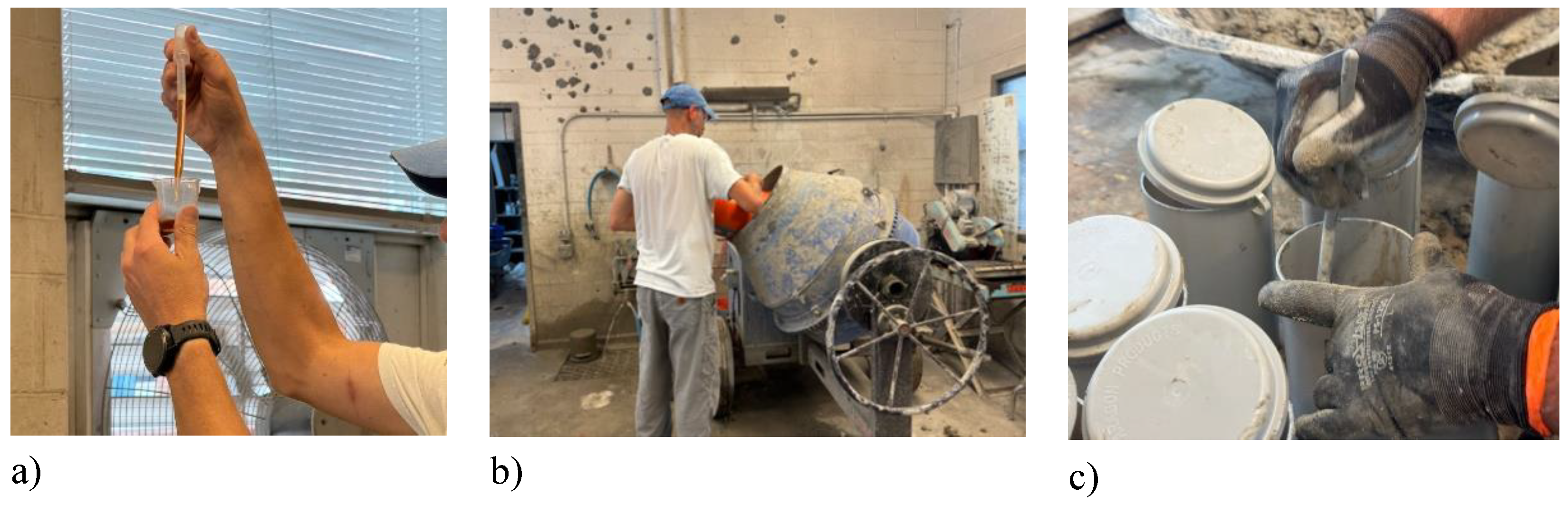
Figure 2.
Conditioning samples a) Wet dry shelving b) Environmental chamber c) Samples in freeze thaw chamber.
Figure 2.
Conditioning samples a) Wet dry shelving b) Environmental chamber c) Samples in freeze thaw chamber.
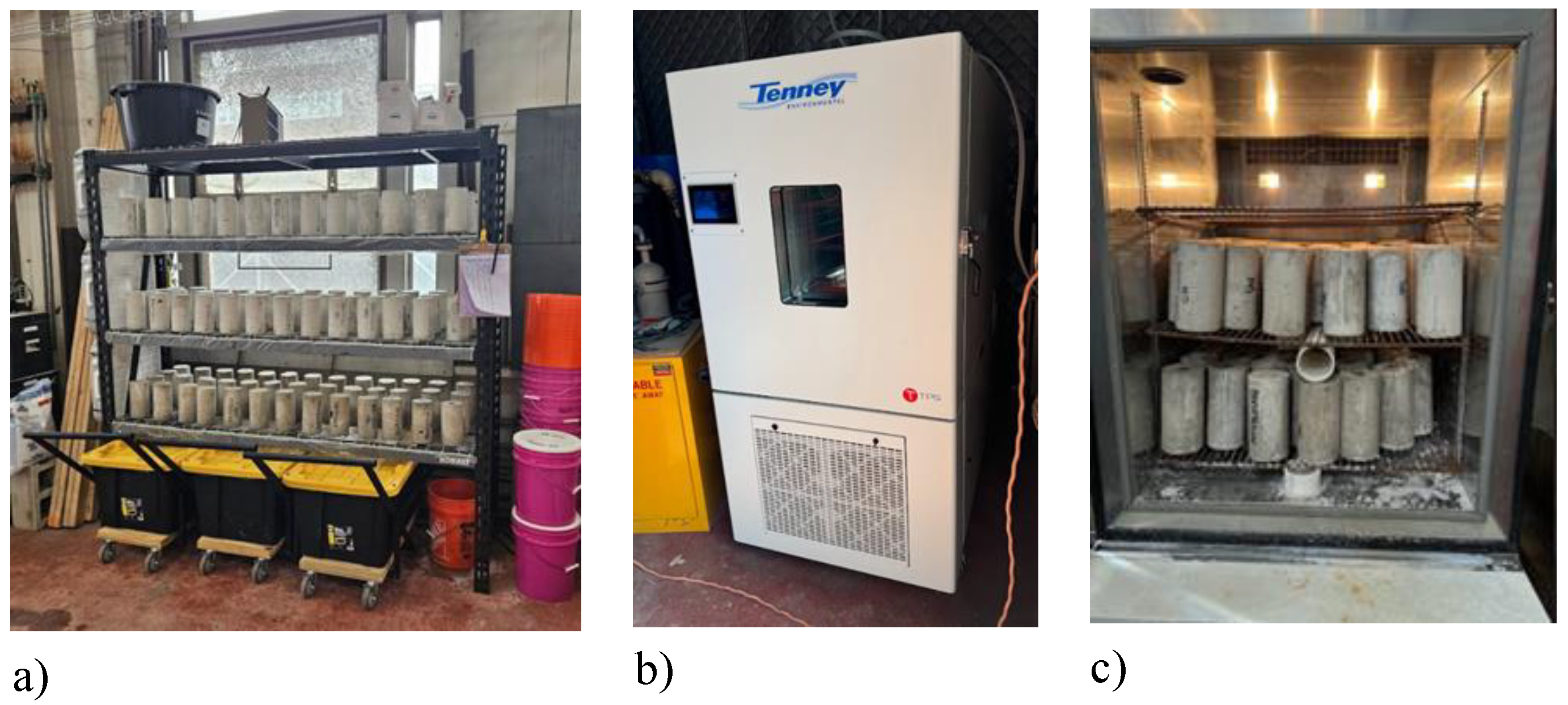
Figure 3.
Bridge core samples a) bagged bridge core from DelDOT b) bridge cores before c) after capping d) Humboldt compression machine.
Figure 3.
Bridge core samples a) bagged bridge core from DelDOT b) bridge cores before c) after capping d) Humboldt compression machine.
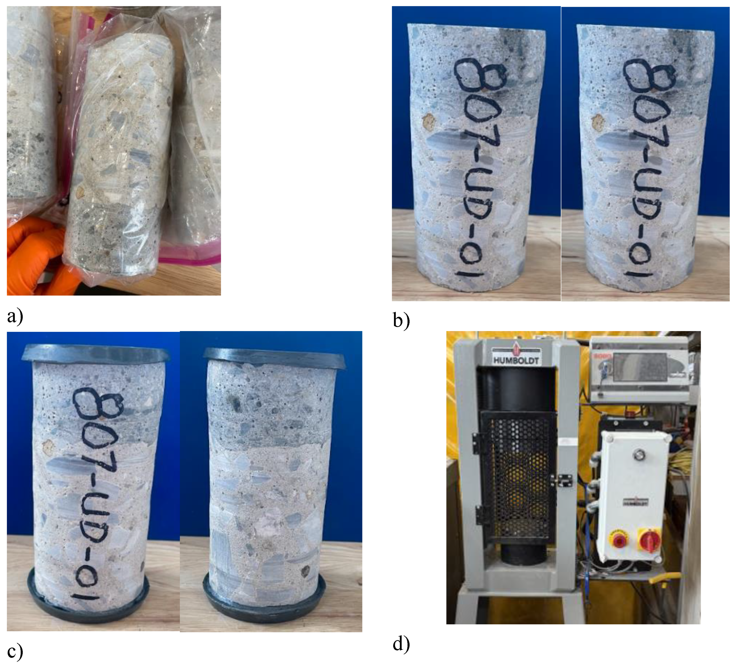
Figure 4.
Resonance frequency testing: (a) experimental setup with concrete cylinder, accelerometer, and data acquisition system, (b) schematic diagram for longitudinal mode testing (After [26]).
Figure 4.
Resonance frequency testing: (a) experimental setup with concrete cylinder, accelerometer, and data acquisition system, (b) schematic diagram for longitudinal mode testing (After [26]).
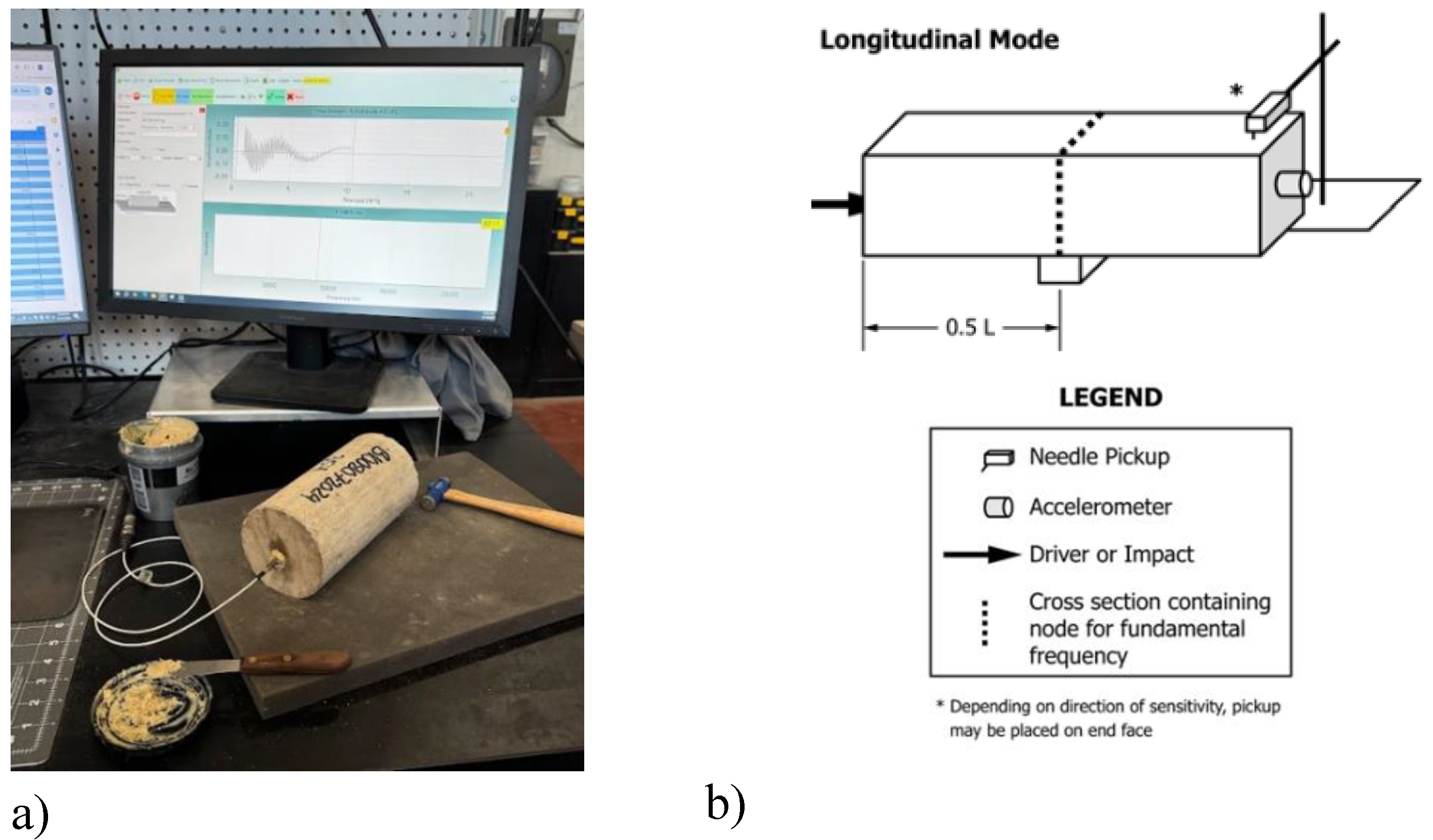
Figure 5.
Broken sample after compression testing b) Bagged sample after compression testing.
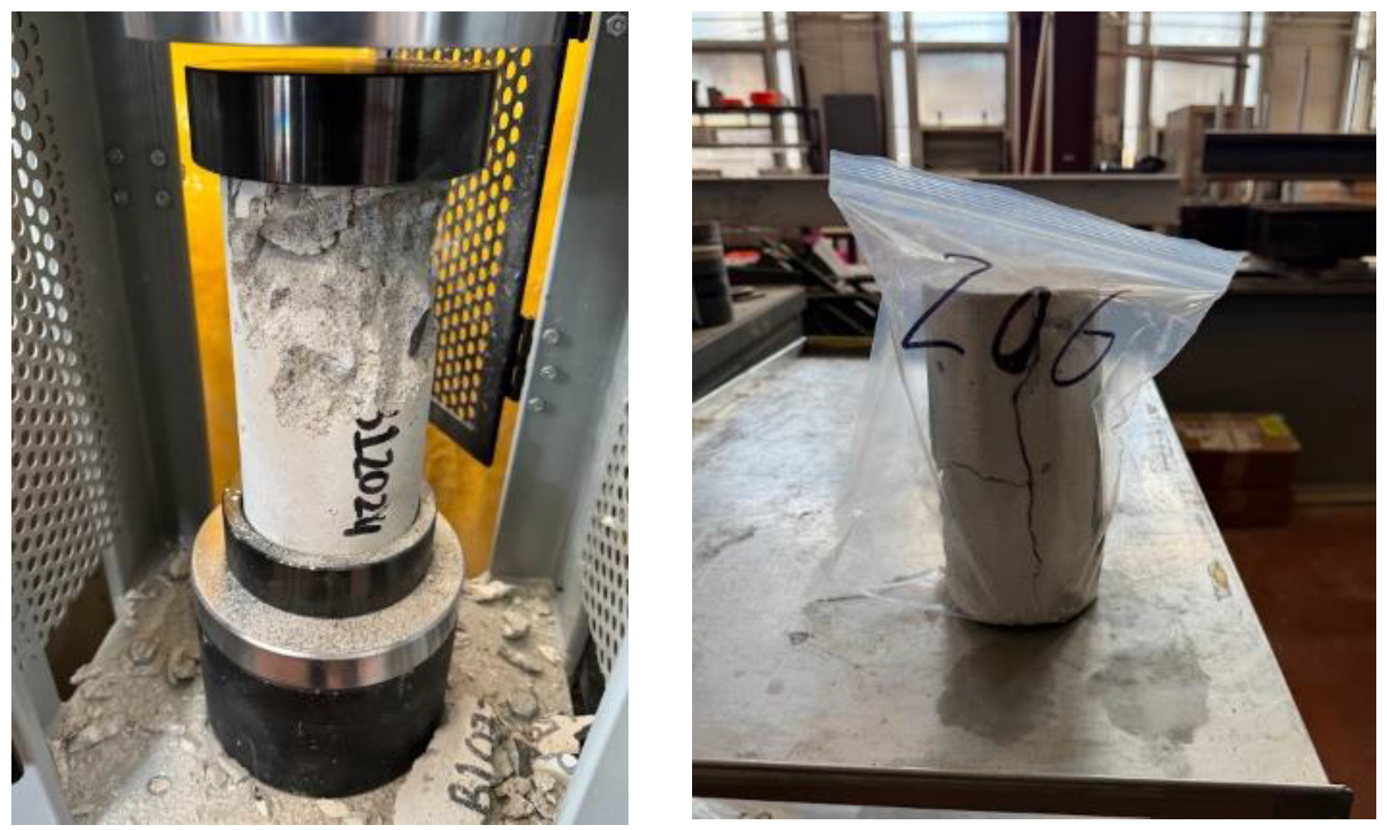
Figure 6.
Humboldt Compressometer /Extensometer.
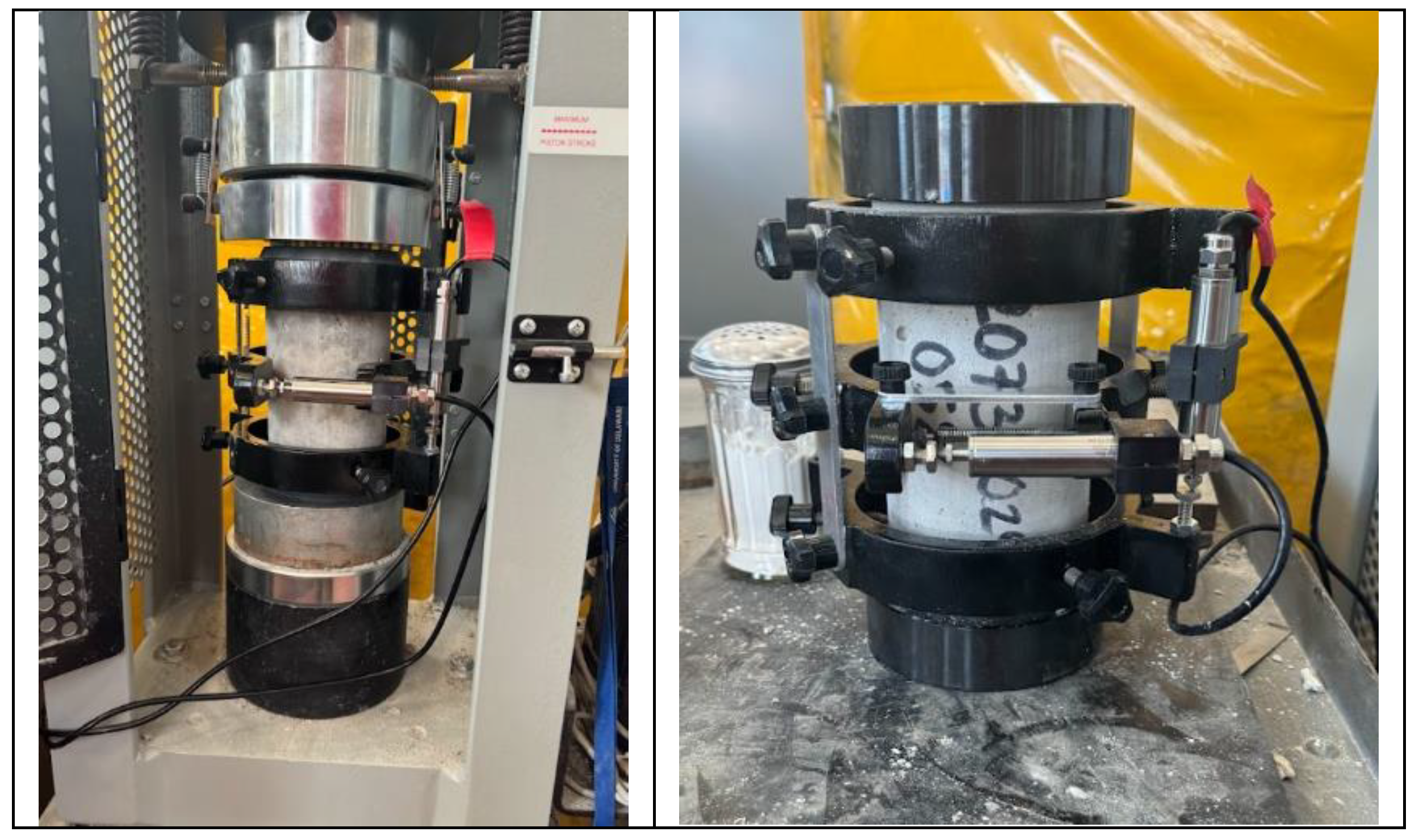
Figure 7.
Resistivity test a) Rock crusher crushing concrete powder b) Weighing concrete powder c) Handheld salinity meter.
Figure 7.
Resistivity test a) Rock crusher crushing concrete powder b) Weighing concrete powder c) Handheld salinity meter.
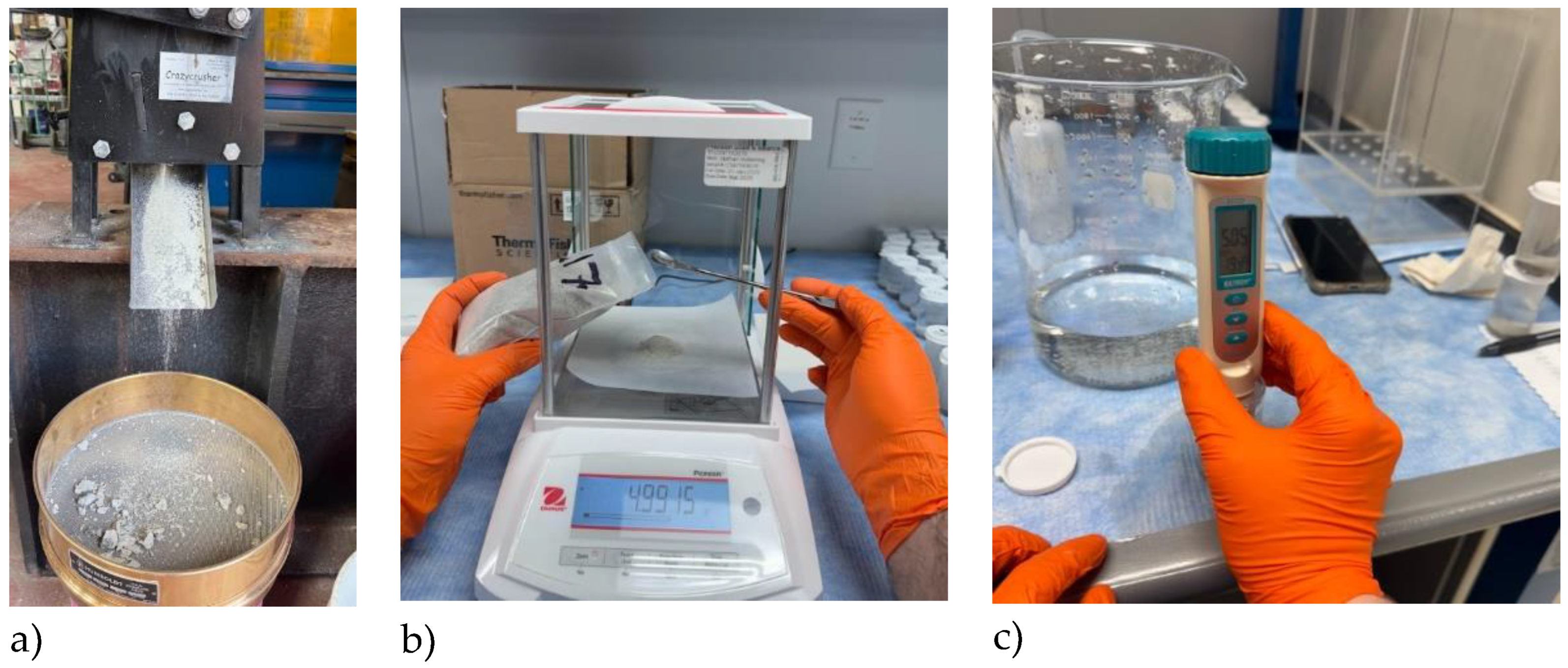
Figure 8.
Wet-Dry Resonance Frequency Cycling – a) 0%, b) 3%, and c) 15%.
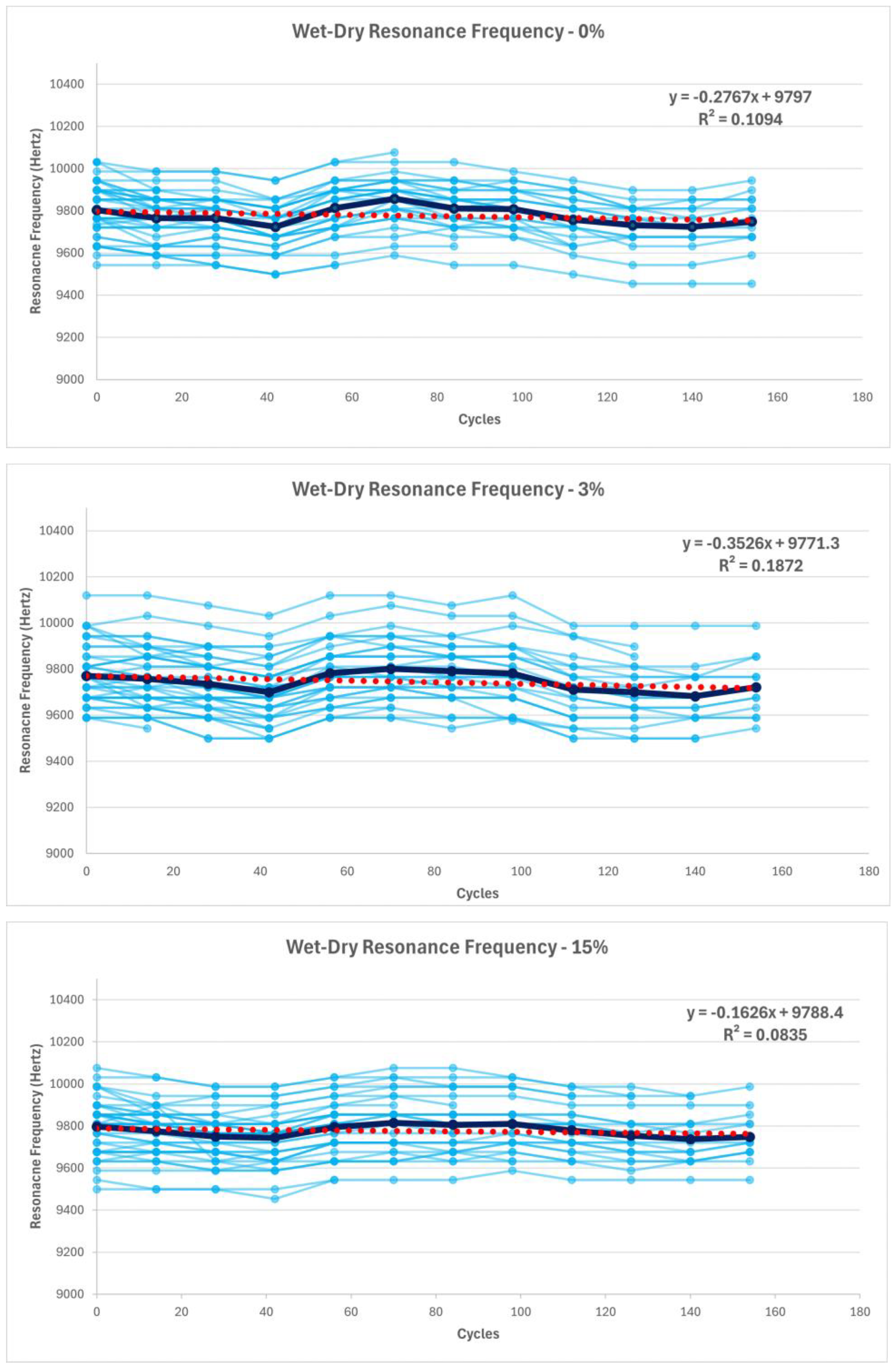
Figure 9.
Freeze-Thaw Resonance Frequency Cycling – a) 0%, b) 3%, and c) 15%.
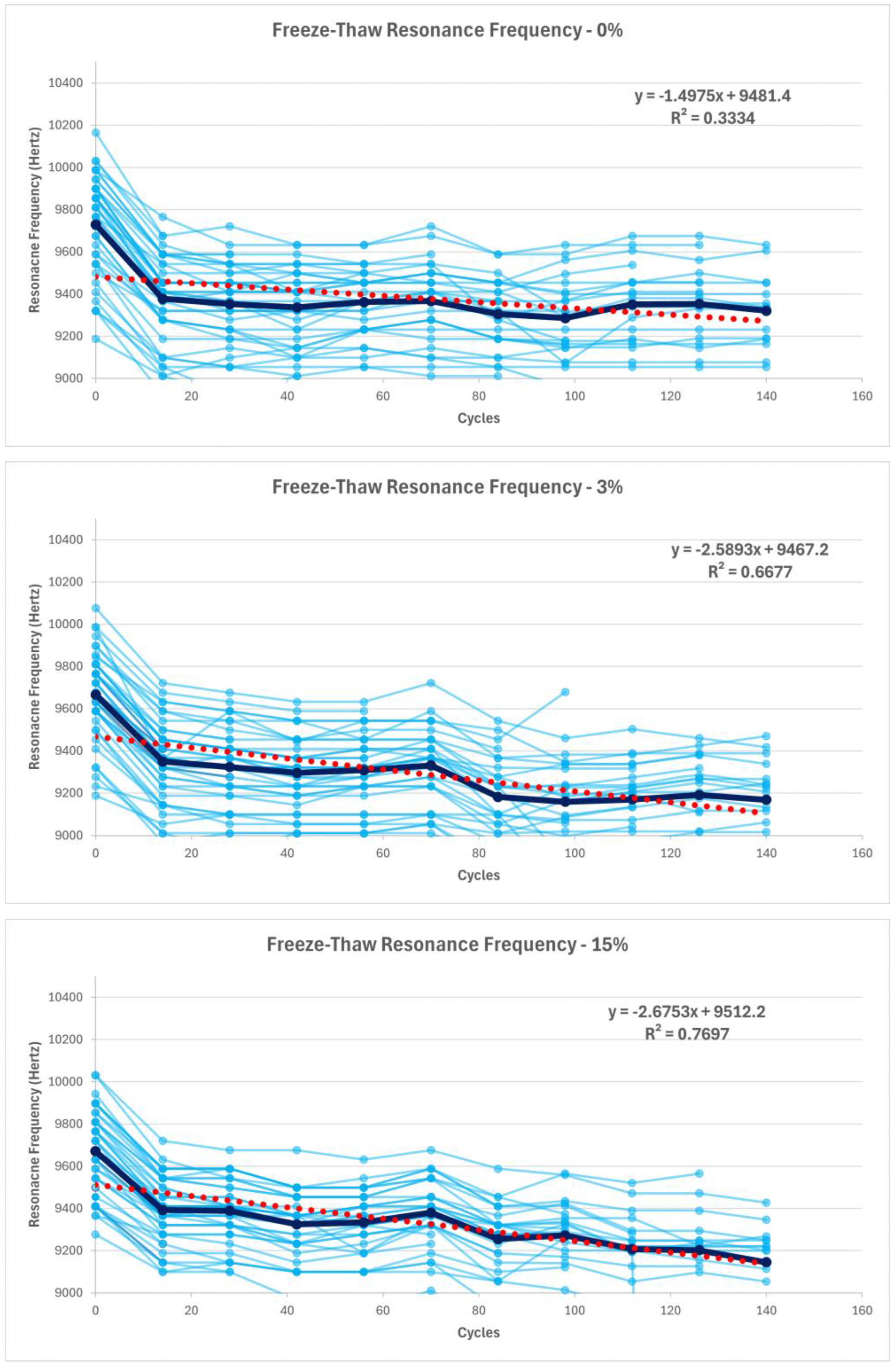
Figure 10.
Control Resonance Frequency Cycling.
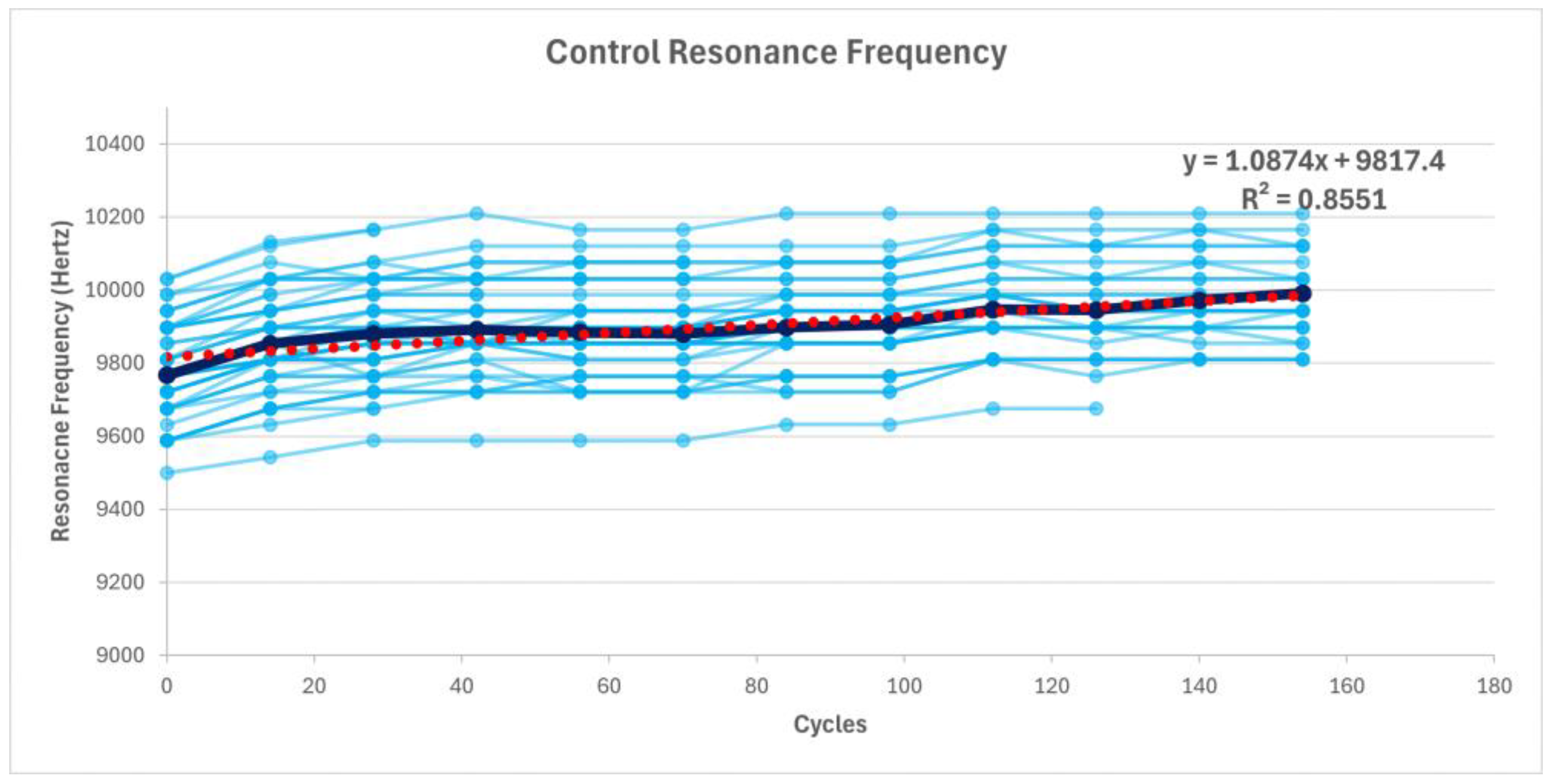
Figure 11.
Compressive Strength Results – a) Wet-Dry Cycling, b) Freeze-Thaw Cycling, and c) Control.
Figure 11.
Compressive Strength Results – a) Wet-Dry Cycling, b) Freeze-Thaw Cycling, and c) Control.
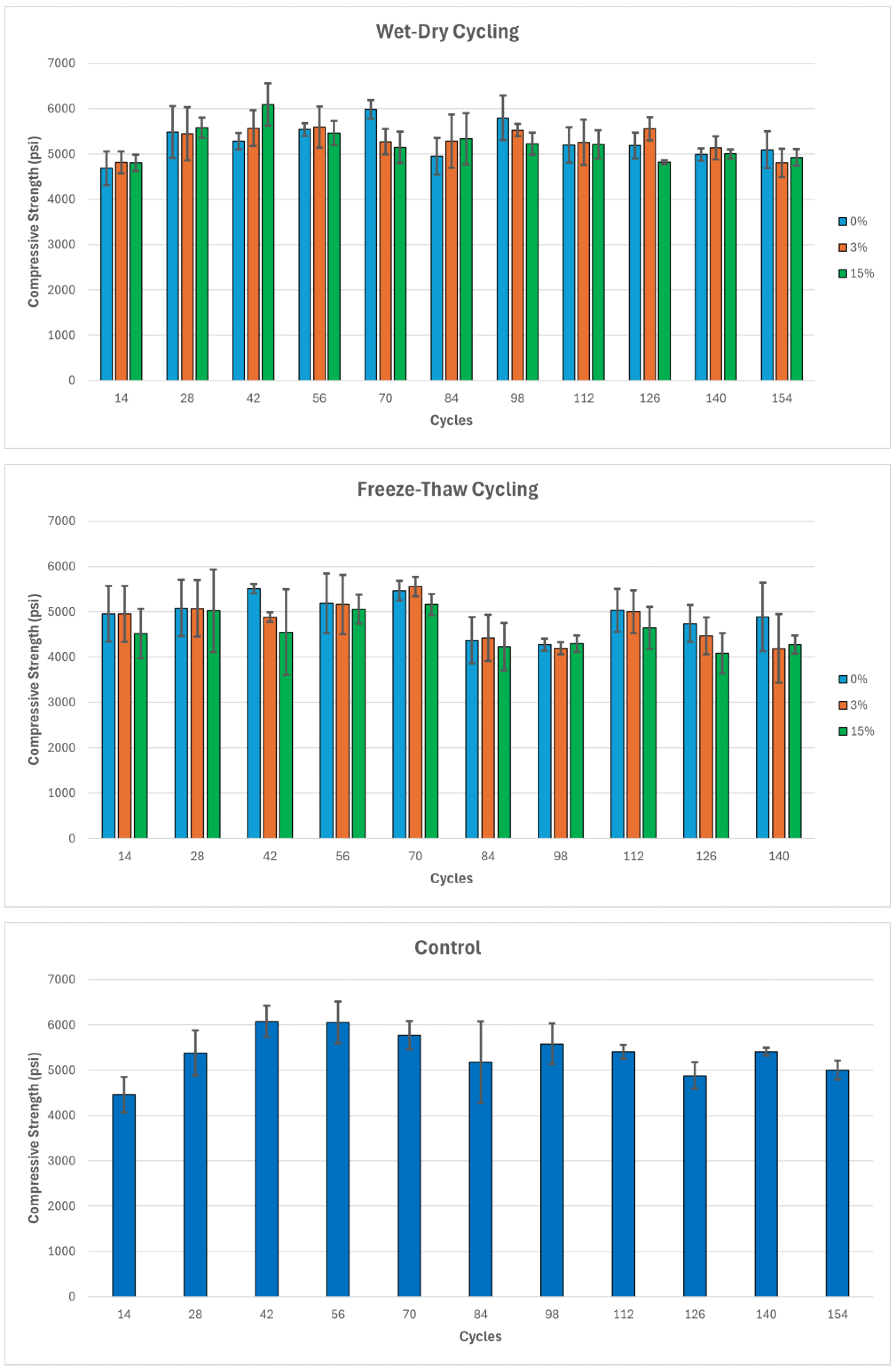
Figure 12.
Modulus of Elasticity Results – a) Wet-Dry Cycling, b) Freeze-Thaw Cycling, and c) Control.
Figure 12.
Modulus of Elasticity Results – a) Wet-Dry Cycling, b) Freeze-Thaw Cycling, and c) Control.
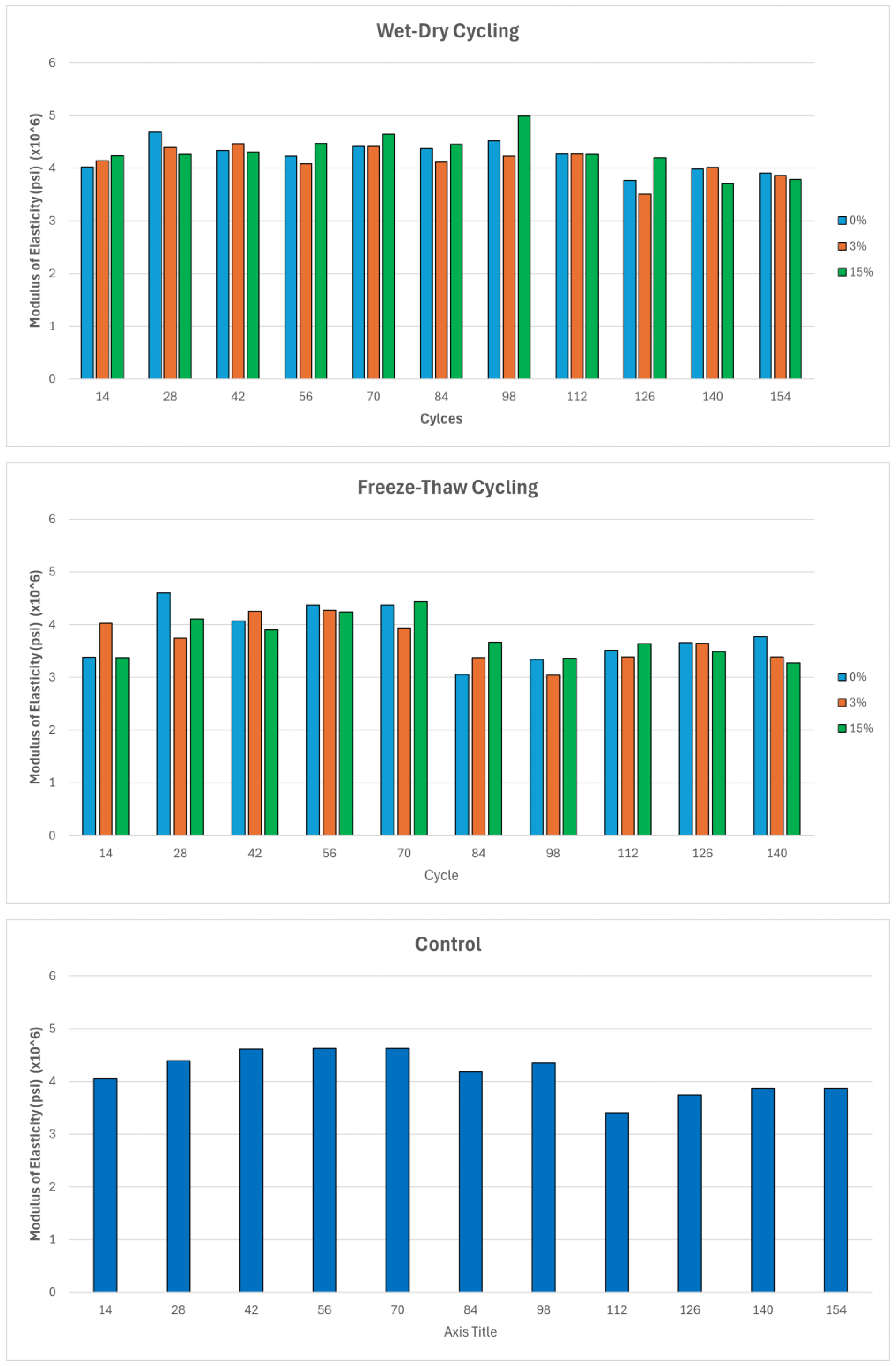
Figure 13.
Poisson's Ratio Results – a) Wet-Dry Cycling, b) Freeze-Thaw Cycling, and c) Control.
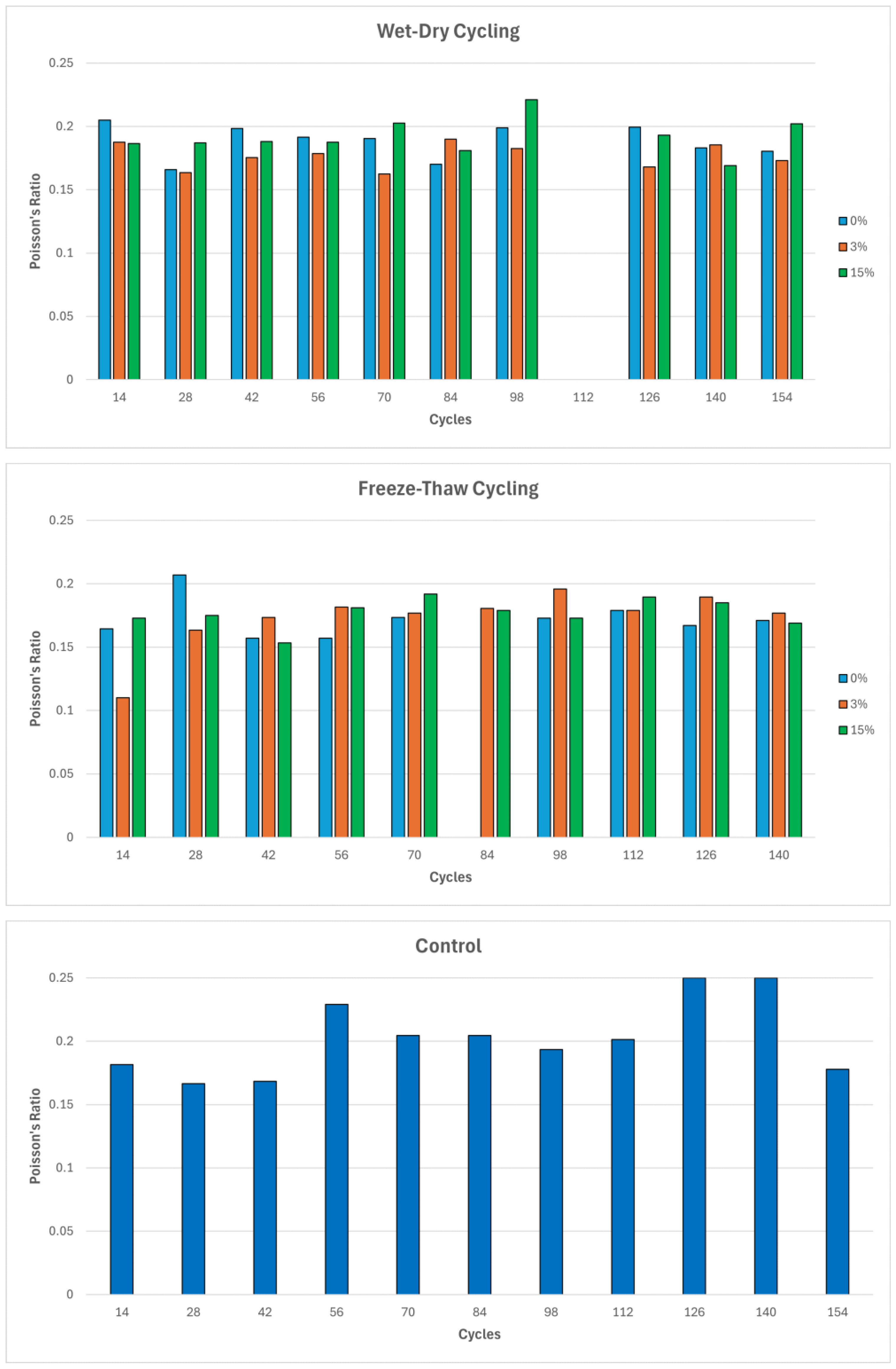
Figure 14.
Chloride Content Results – a) Wet-Dry Cycling, b) Freeze-Thaw Cycling, and c) Control.
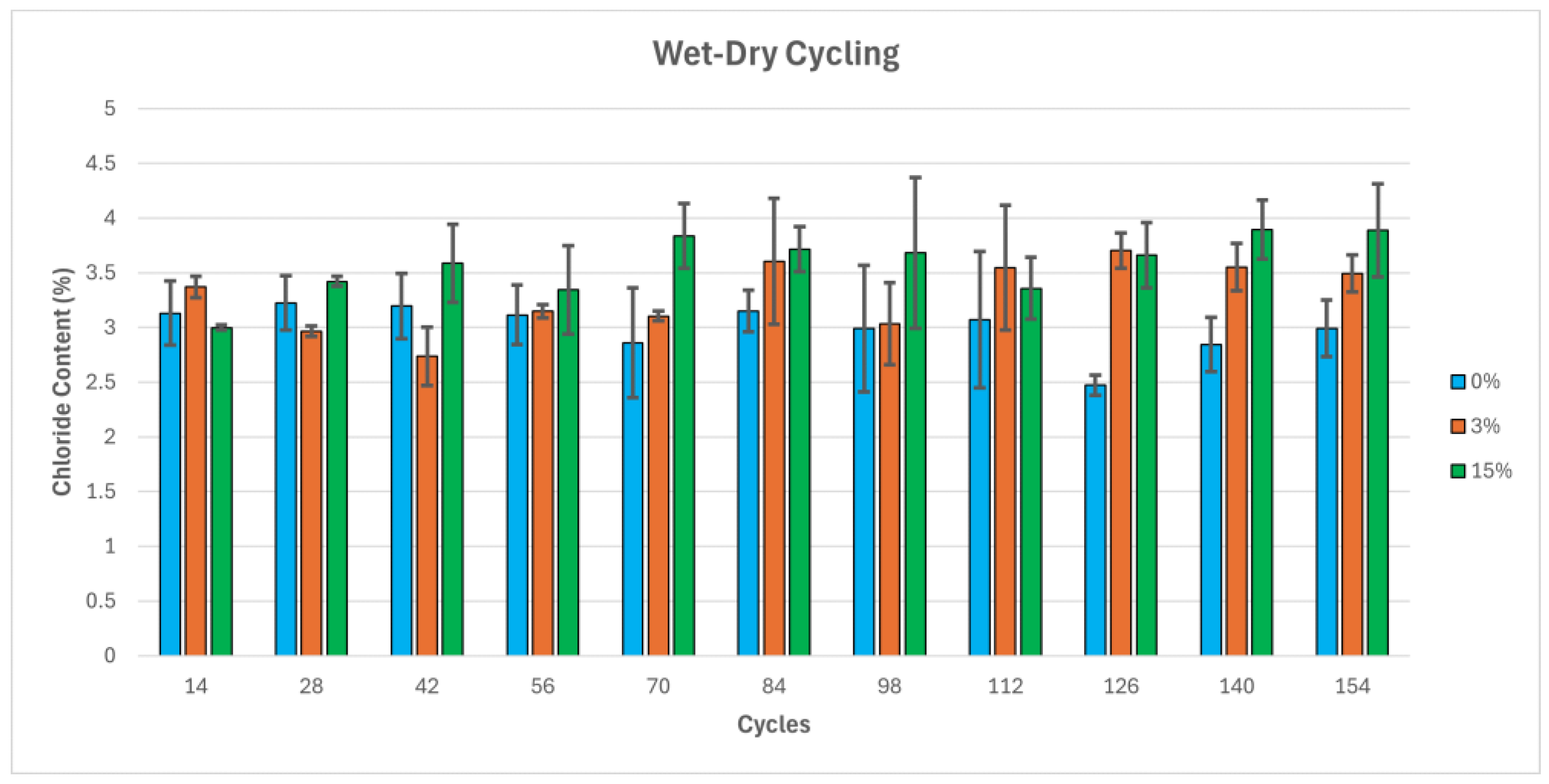
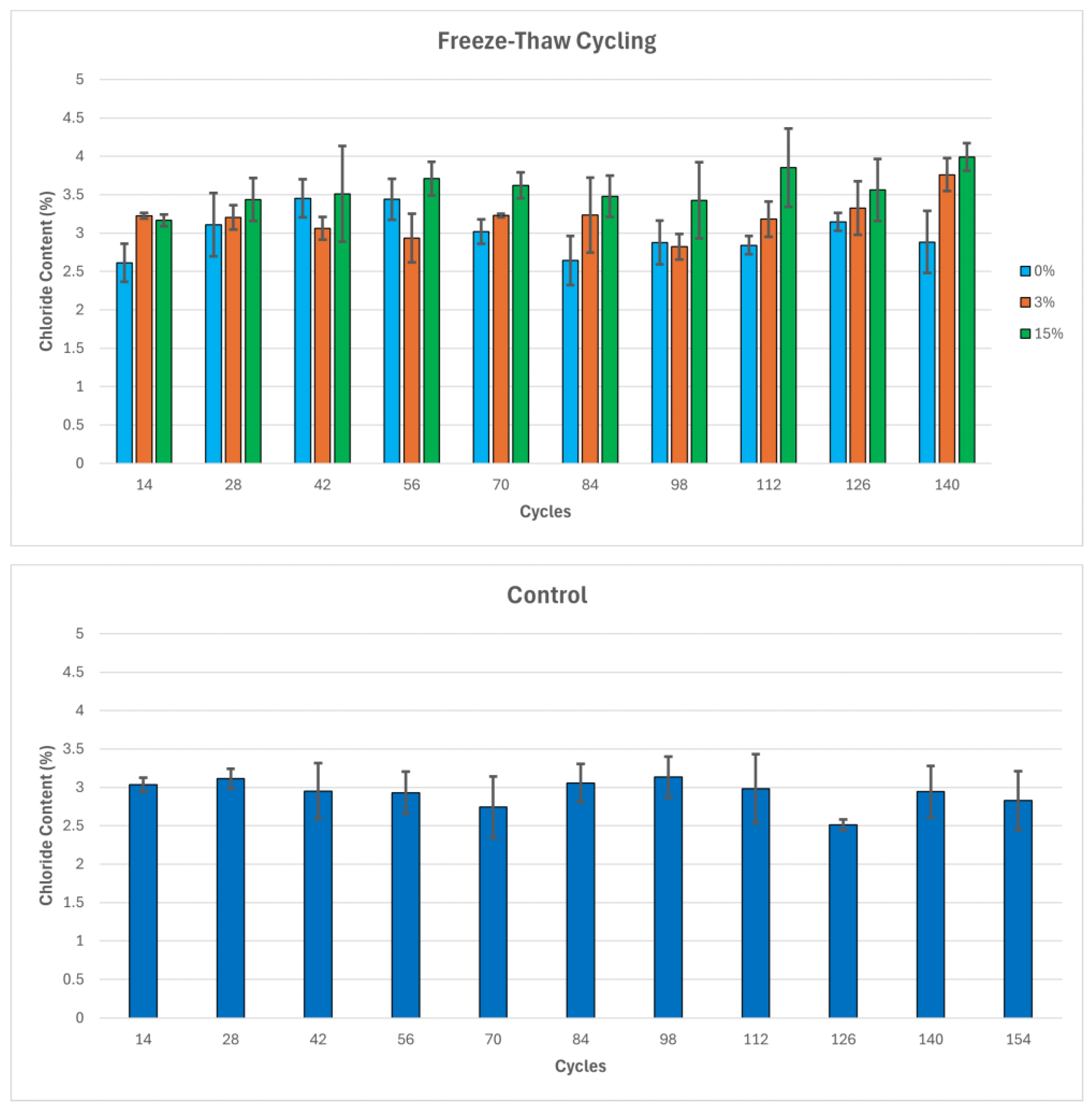
Figure 15.
I-495 Viaduct Bridge Locations.
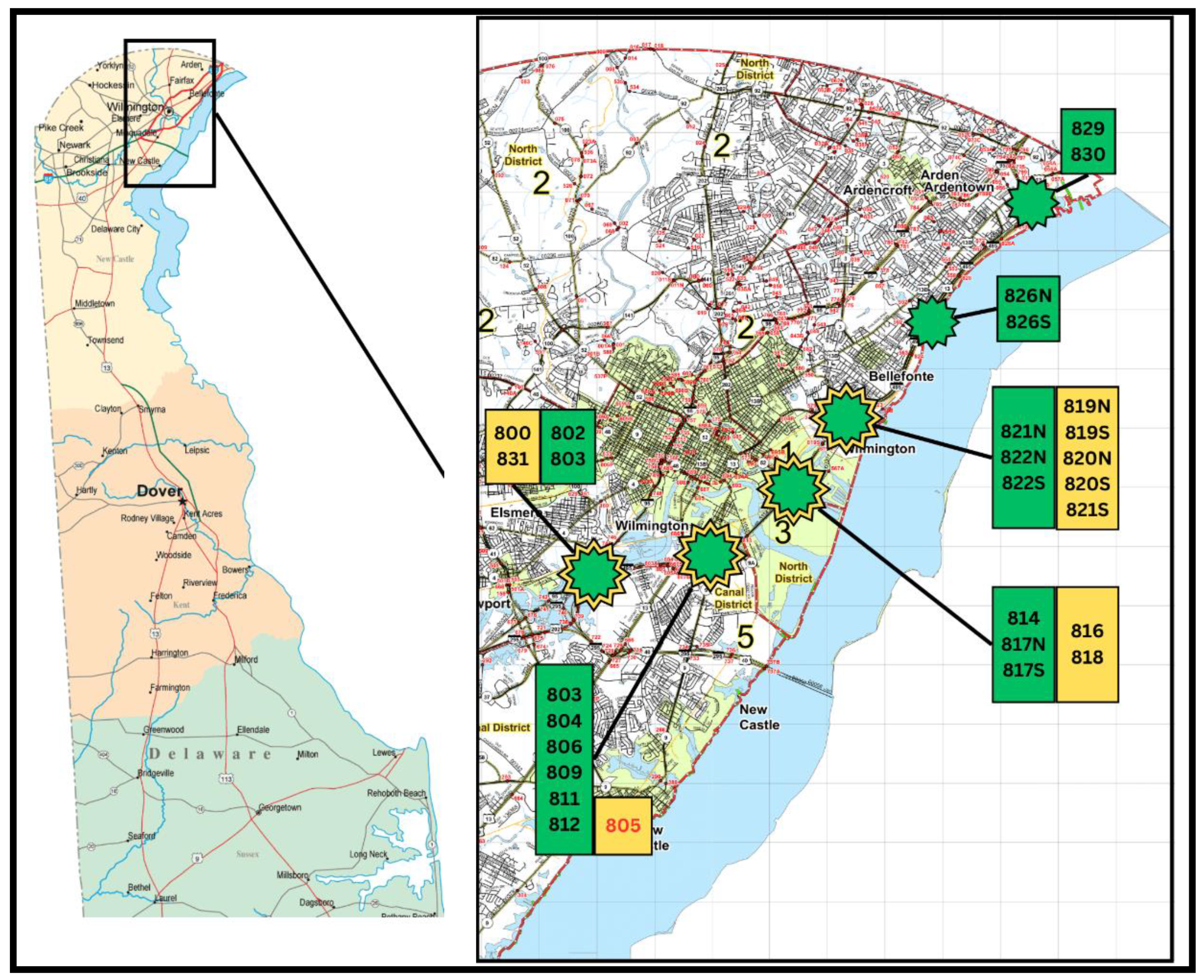
Figure 16.
DelDOT Bridge Condition Dashboard.
Figure 17.
Age of Bridges Examined.
Figure 18.
Bridge Deck Core Compressive Strength.
Figure 19.
Compressive Strength Breakdown by Age.
Figure 20.
Chloride Content Breakdown by Age.
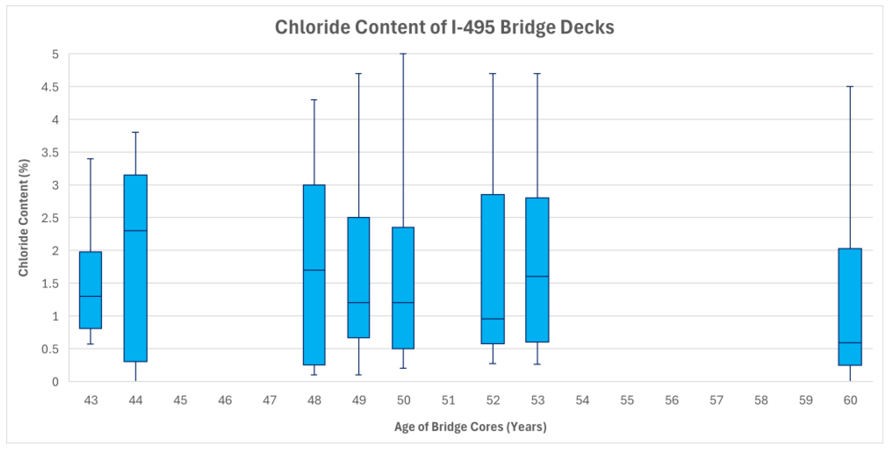
Figure 21.
Predicted Versus Counted Freeze Thaw Cycles.
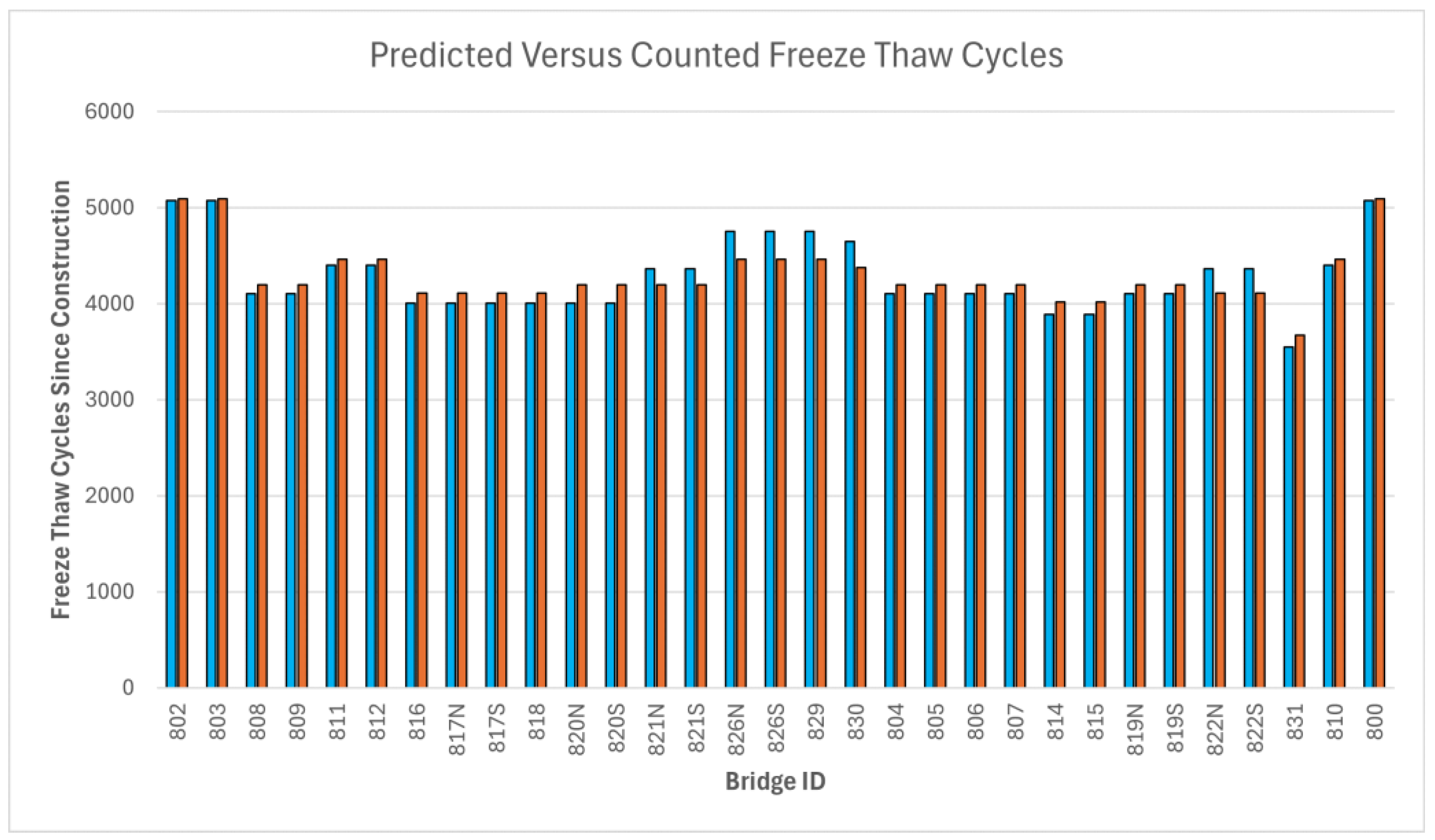
Figure 22.
92 Years of NOAA Weather Data for Wilmington, DE.
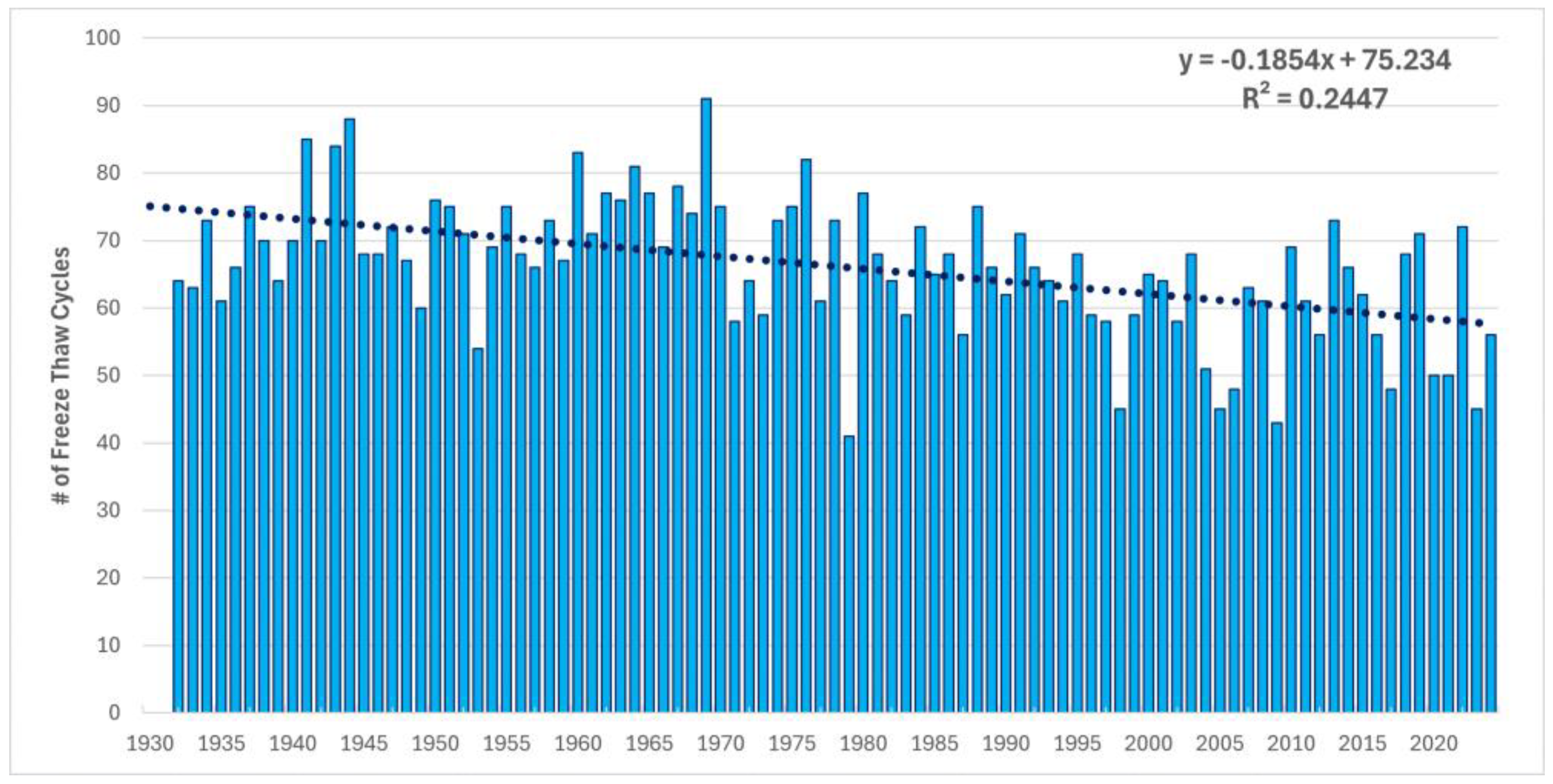
Figure 23.
Number of Snowfall Days per Year.
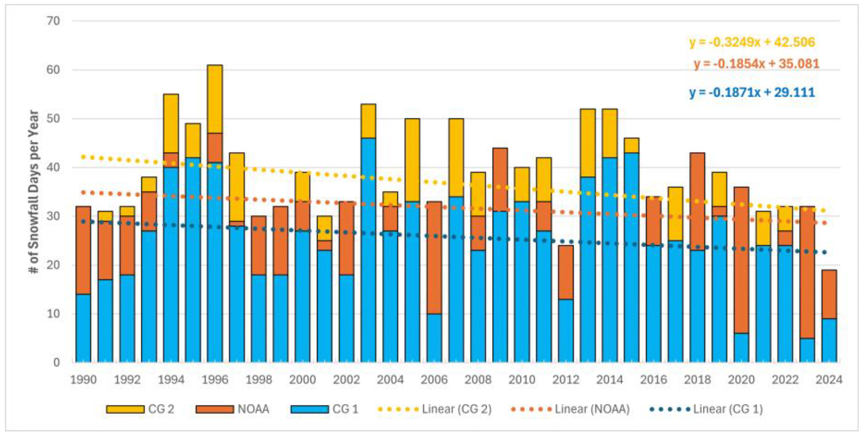
Figure 24.
Average Resonance Frequency of Lab Samples.
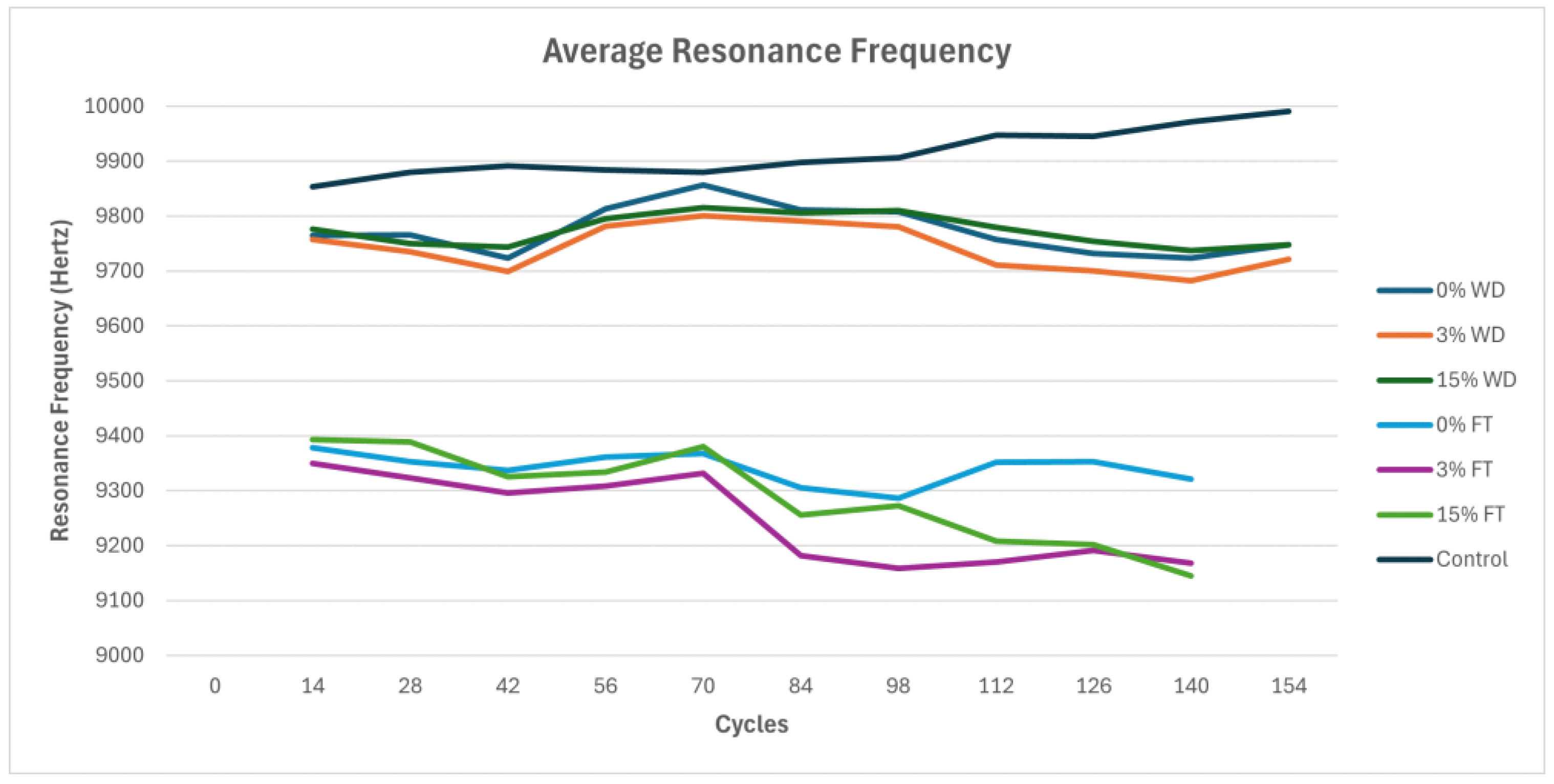
Figure 25.
Linear Trendline of Lab Samples.
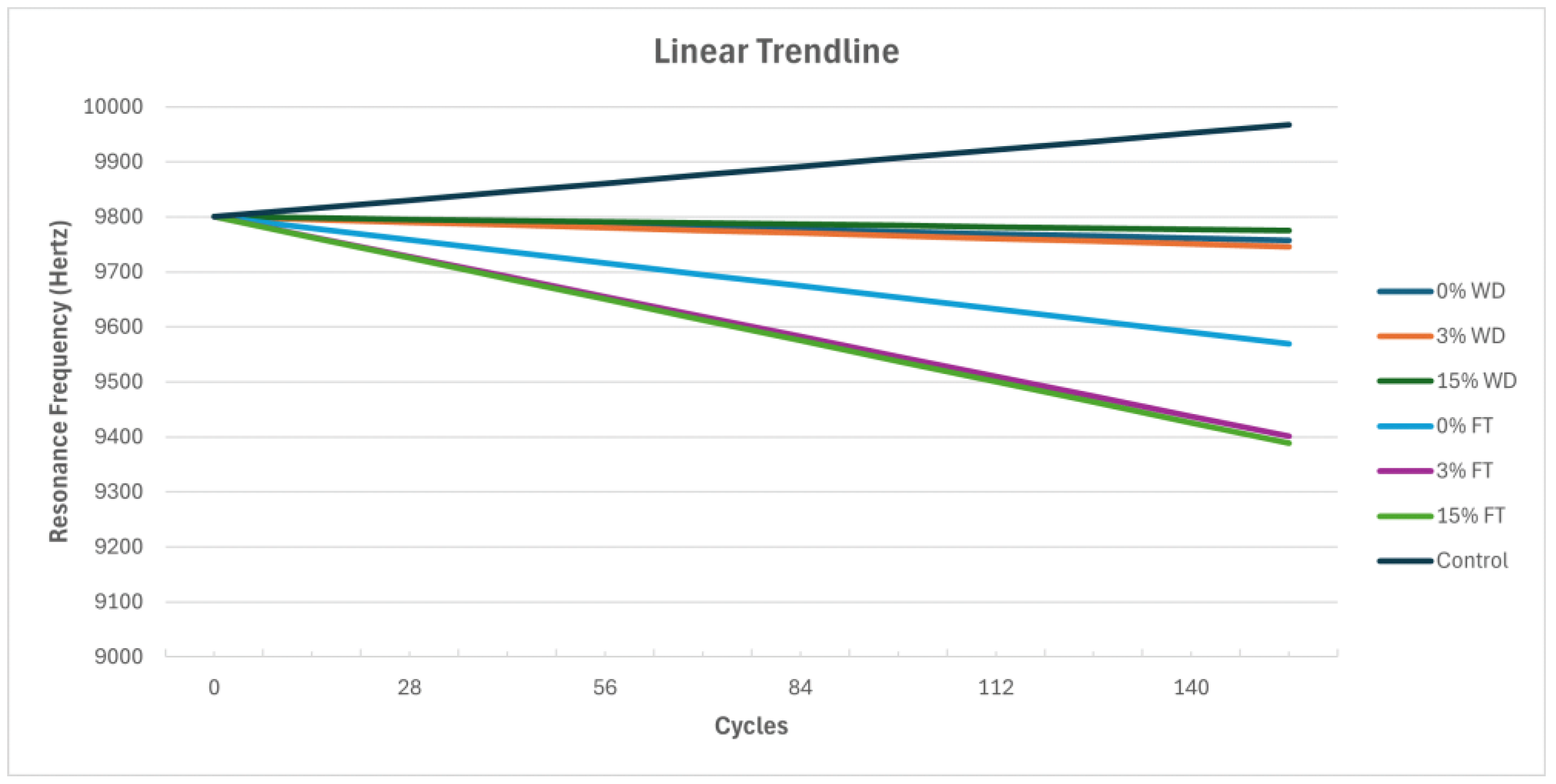
Figure 26.
Compressive Trends of Experimental Samples - a) Wet-Dry Cycling, b) Freeze-Thaw Cycling, and c) Control.
Figure 26.
Compressive Trends of Experimental Samples - a) Wet-Dry Cycling, b) Freeze-Thaw Cycling, and c) Control.
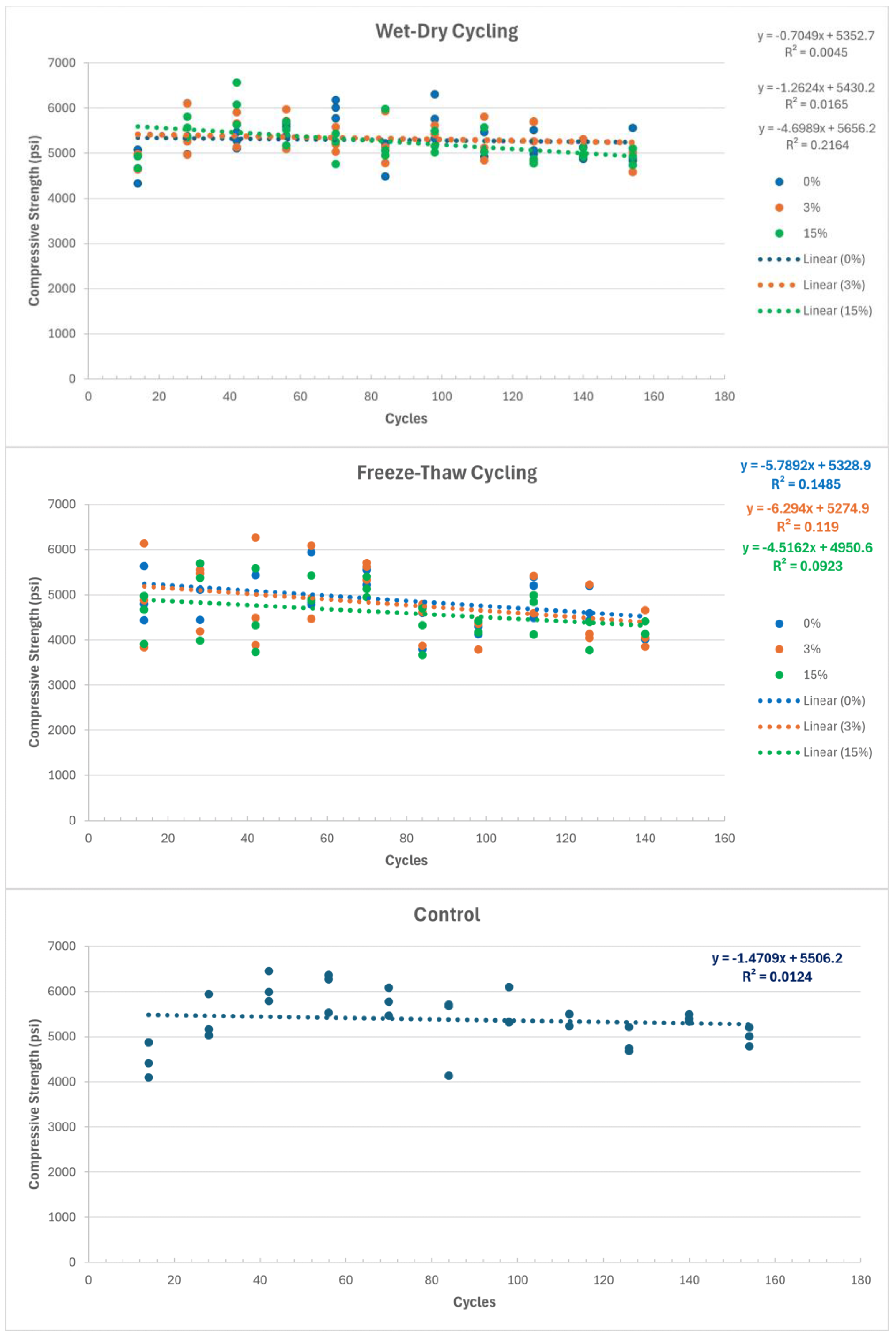
Figure 27.
Chloride Trends of Experimental Samples, a) Wet-Dry Cycling and b) Freeze-Thaw Cycling.
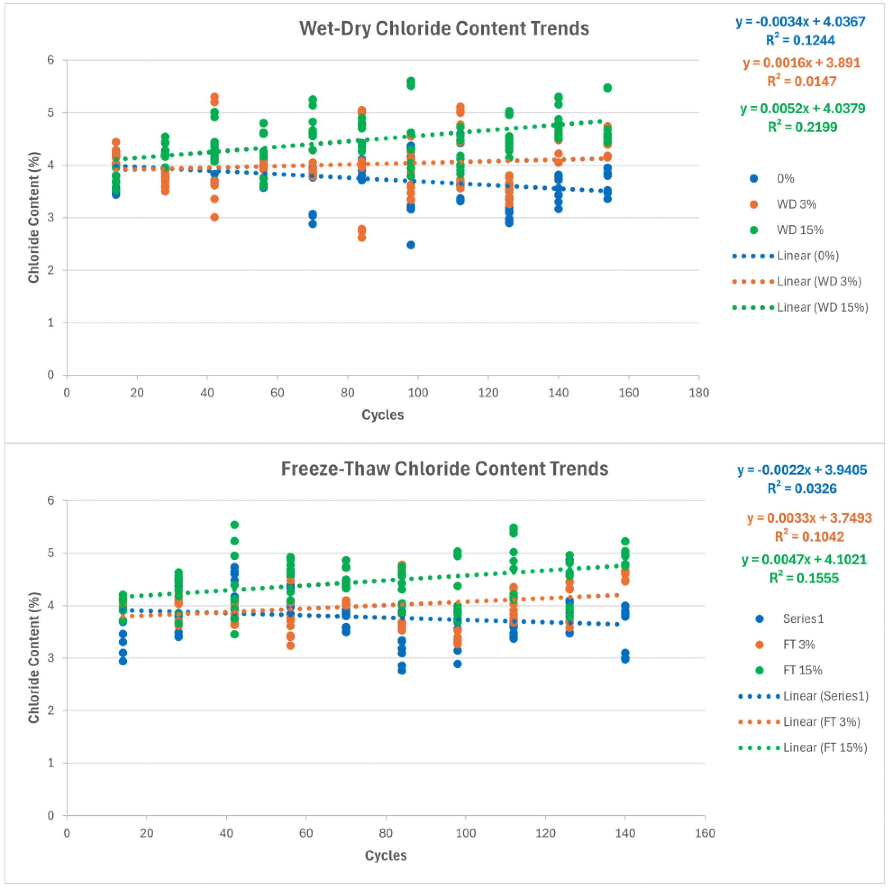
Figure 28.
Resonance Frequency and Compressive Trends Comparison - a) Wet-Dry Cycling, b) Freeze-Thaw Cycling, and c) Control.
Figure 28.
Resonance Frequency and Compressive Trends Comparison - a) Wet-Dry Cycling, b) Freeze-Thaw Cycling, and c) Control.
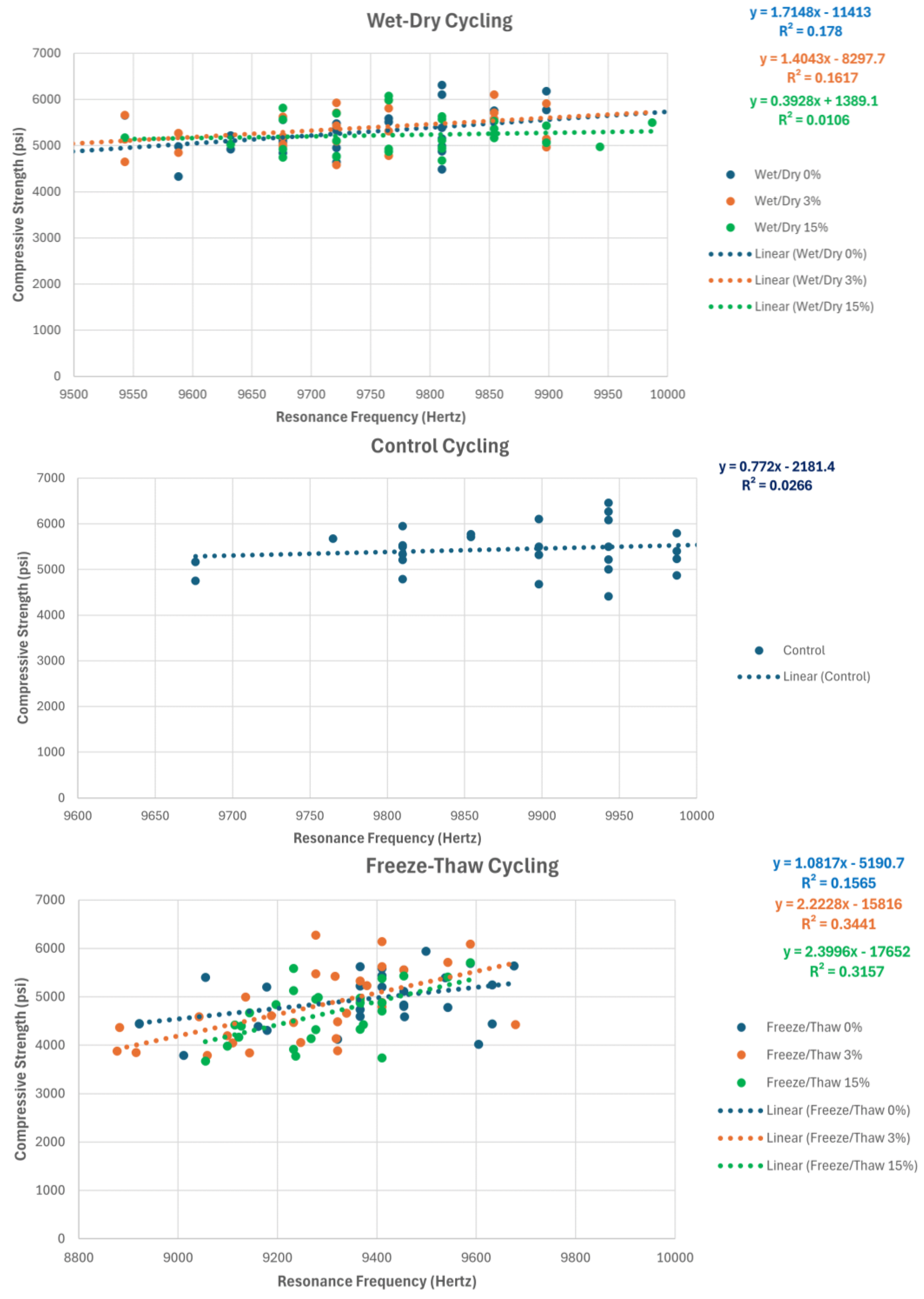
Figure 29.
Predictive Equations Compared Against Experimental Data.
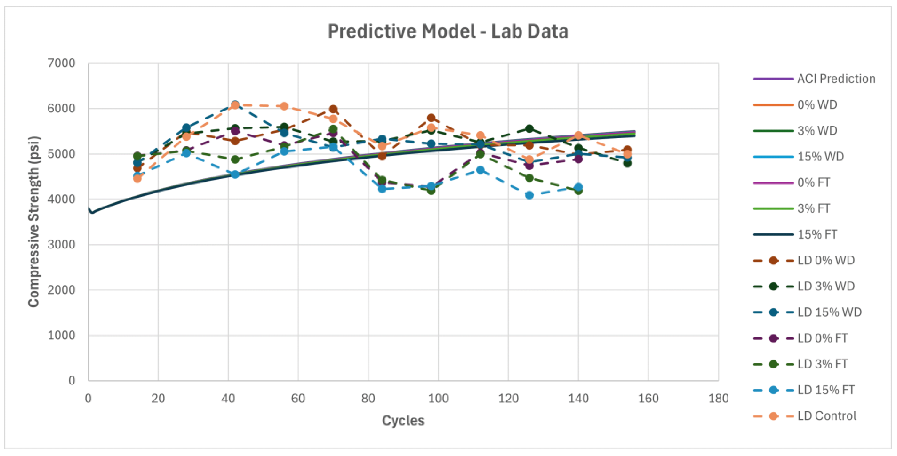
Figure 30.
Chloride Predictive Model With I-495 Bridge Core Concentrations.
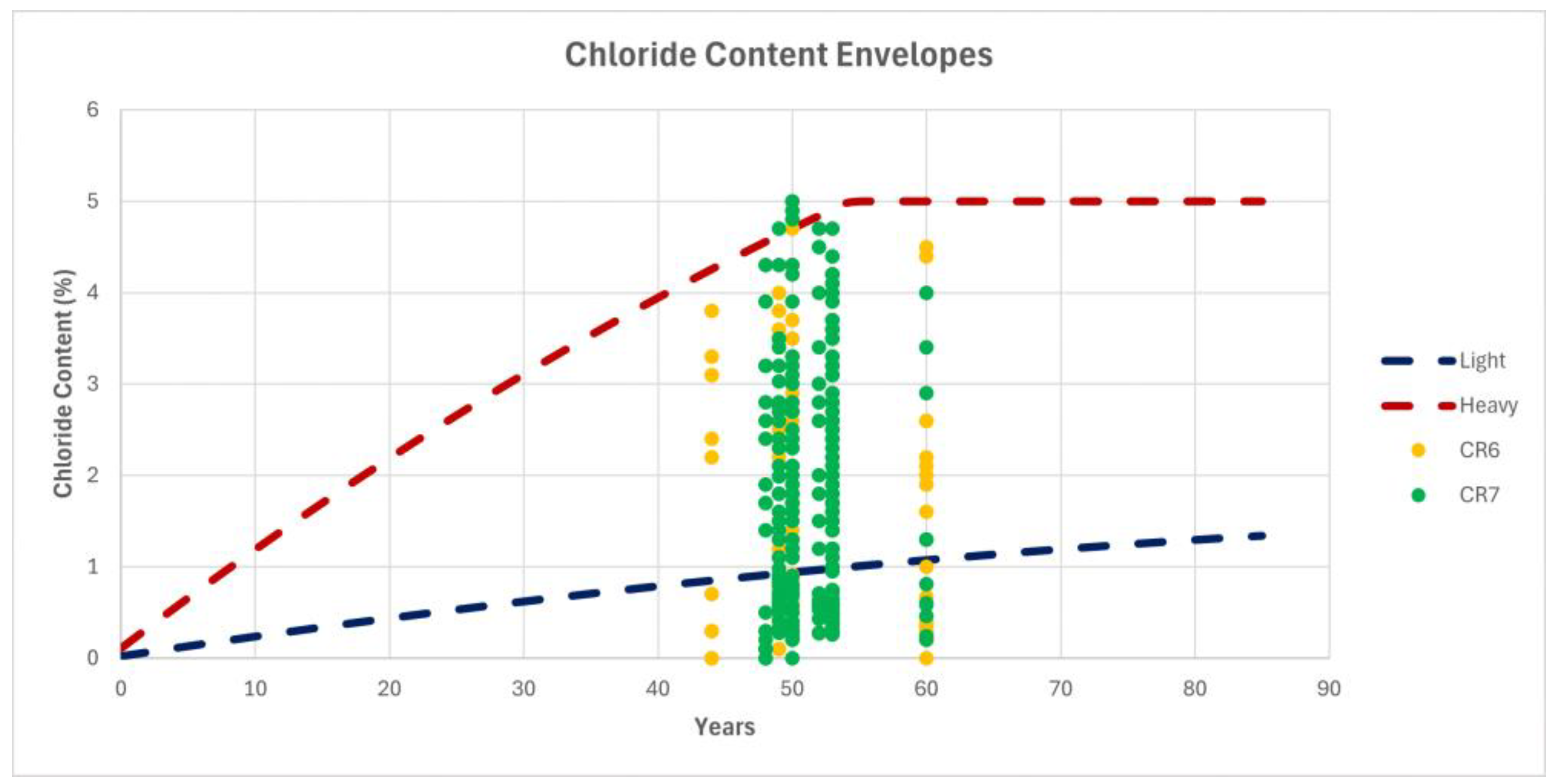
Figure 31.
Deterioration Envelope With I-495 Bridge Core Compressive Strengths.
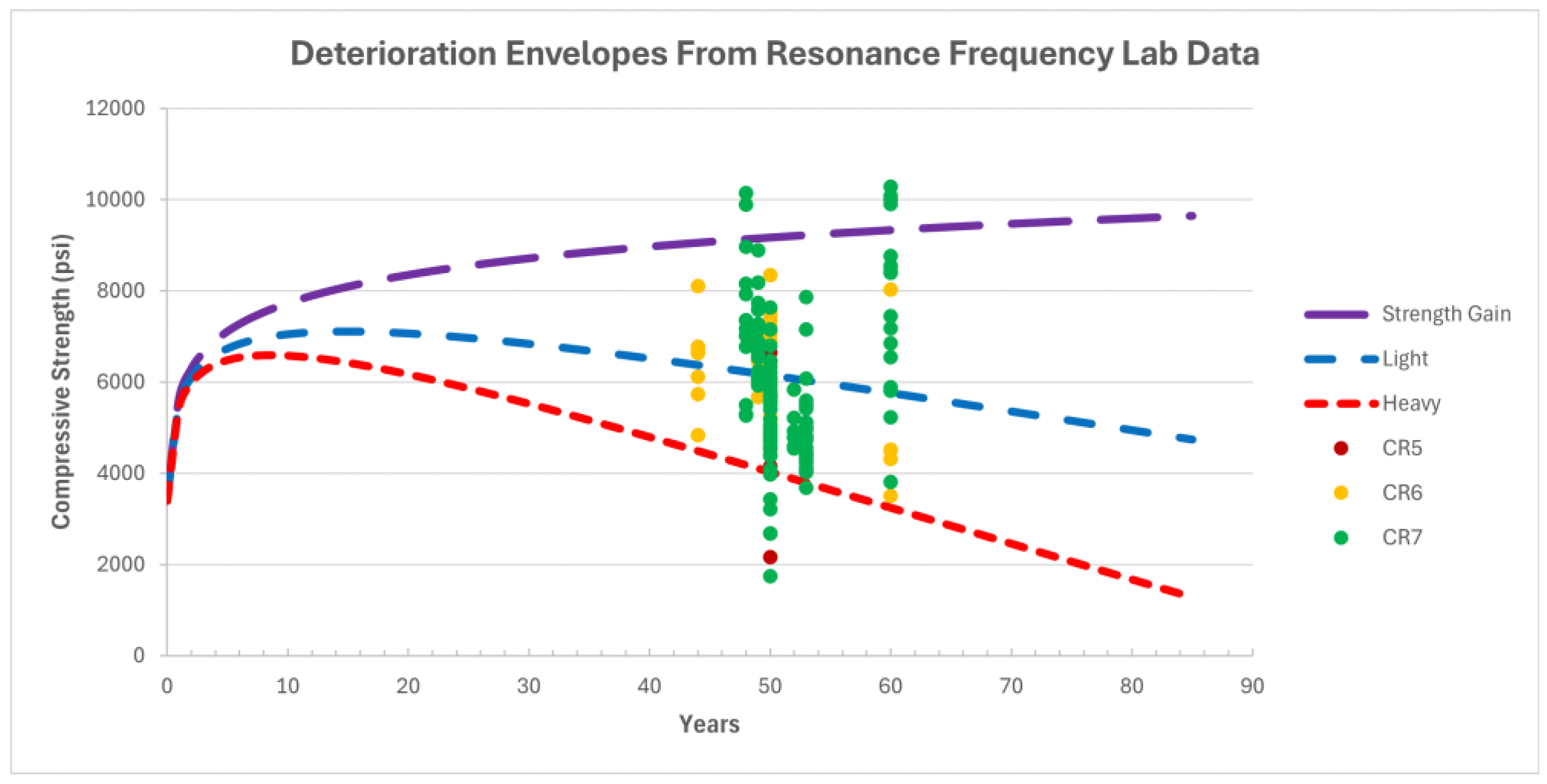
Figure 32.
Durability Index of I-495 Bridges.
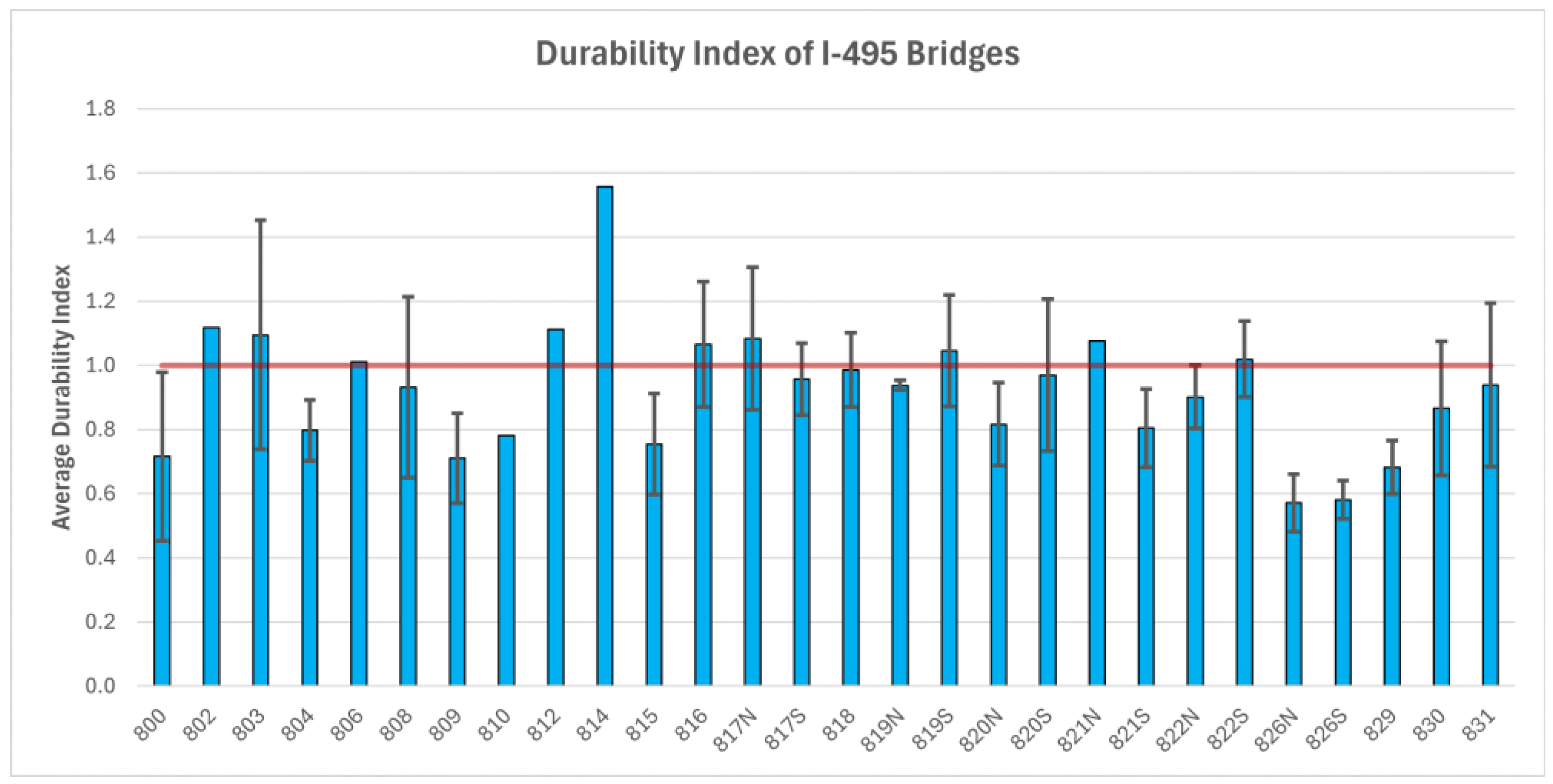

Table 1.
Concrete Mix Design for Historic Mix.
| Parameter | Value | Selection Rationale |
|---|---|---|
| Cement Specific Gravity | 3.15 | Standard value |
| Coarse Aggregate Specific Gravity | 2.7 | From documentation |
| Fine Agg Specific Gravity | 2.65 | From lab testing of material |
| Coarse Agg Dry Unit Wt. (Unit) | 99.6 | From lab testing of material |
| Coarse Agg Moisture Content (%) | 1 | Found prior to batching |
| Fine Agg Moisture Content (%) | 1 | Found prior to batching |
| Slump [mm.] | 127 | Design Selection |
| Air Content (%) | 6 | Design Selection |
| Compressive Strength [MPa] | 25 | Design Selection |
| Slump/max Aggregate | 305 | |
| Compressive Strength w/c | 0.4 | |
| Max Agg/Fine Mod | 0.6 | |
| Coarse Agg Volume [CBM] | 0.46 | |
| Coarse Agg Weight [kg] | 732 | Based on Dry Rodded Unit Weight |
| Density of water [kg/m3] | 1000 | At room temperature |
| Water Weight [kg] | 99.7 | From w/c ratio |
| Volume of water [CBM] | 3.77 | Calculated based on density |
| Cement Weight [kg] | 249.5 | From w/c ratio |
| Volume of Cement [CBM] | 0.079 | Calculated based on density |
| Volume of Coarse Agg [CBM] | 0.27 | Calculated based on density |
| Air Volume [CBM] | 0.046 | Calculated based on air content requirement |
| Total Volume [CBM] | 0.52 | |
| Fine Agg Volume [CBM] | 0.24 | Calculated based on remaining volume in 1 cu. yd. |
| Fine Agg Weight [kg.] | 638.88 | Calculated based on density |
| Stockpile [CBM] | [kg/CBM] | [kg/CBM] |
| Fine Agg Batch Weight [kg] | 645.27 | 60.53 |
| Coarse Agg Batch Weight [kg] | 739.2 | 69.35 |
| Cement Batch Weight [kg] | 249.5 | 23.4 |
| Water Batch Weight [kg] | 101.7 | 9.54 |
| Total Batch Weight [kg] | 1735.65 | 162.82 |
Disclaimer/Publisher’s Note: The statements, opinions and data contained in all publications are solely those of the individual author(s) and contributor(s) and not of MDPI and/or the editor(s). MDPI and/or the editor(s) disclaim responsibility for any injury to people or property resulting from any ideas, methods, instructions or products referred to in the content. |
© 2025 by the authors. Licensee MDPI, Basel, Switzerland. This article is an open access article distributed under the terms and conditions of the Creative Commons Attribution (CC BY) license (http://creativecommons.org/licenses/by/4.0/).
Copyright: This open access article is published under a Creative Commons CC BY 4.0 license, which permit the free download, distribution, and reuse, provided that the author and preprint are cited in any reuse.


