
Submitted:
04 December 2025
Posted:
05 December 2025
You are already at the latest version
Abstract
This paper presents the development and validation of a 3D CFD model of a heave plate under forced oscillations using a Lattice-Boltzmann, LES software, which has never been used for industrial applications in this context. The main objective of the model is to be versatile enough to maintain accuracy in extreme cases of amplitudes and frequencies. The validation is carried out with experimental results from previous research, with some results also compared with the ones obtained using a finite-volume software. A lattice and time step convergence is achieved along with a symmetry study. Once the optimal model has been selected it is tested under 4 extreme cases, analyzing the results yielded for the force, added mass and damping coefficients and also assessing its limitations. Results show good correlation between the model and the experimentation, especially in cases of higher force values, and also with the results from the finite-volume software. Further-more, a vorticity field study will be carried out to better understand the behavior of the heave plate in these extreme cases. Finally, an assessment of the dominance of pres-sure-induced forces over viscous forces under low KC numbers is carried out using radial and surface integration.
Keywords:
CFD
; Lattice-Boltzmann Method
; LES
; heave plates
; experimental validation
; ocean engineering
1. Introduction
Floating offshore wind energy has become a reliable way to exploit the potential of the wind resource in deep waters, where more constant and intense winds make it a powerful asset. However, predicting and controlling the dynamic behavior of floating platforms issues an important challenge for marine engineering due to the combined action of waves, sea currents and wind. In this context, heave plates play a main role in improving the platform’s stability thanks to their damping effects both in heave and pitch [1].
Bibliography shows many studies aimed to analyze and improve the design of heave plates in order to optimize their behavior and therefore obtain a better energetic efficiency [2]. To do so, numerical methods such as Computational Fluid Dynamics (CFD) stand as vital tools that enable the study of the hydrodynamic impact of heave plates, aiming to predict their damping and added mass coefficients [3,4] . Nevertheless, computational models always need to be validated with experimental studies [5].
In recent years, heave plate design has significantly evolved. From being employed firstly in oil platforms to reduce their heave response due to waves [6] to their application in FOWTFs due to their ability to improve the dynamic stability and minimize non-desired oscillations [7].
In this sense, recent configurations include circular, rectangular and perforated heave plates. In [8] a combined experimental and numerical study proved that the size and shape of heave plates have a strong influence in the dynamic response of the platform. For example, in [9] and [10] it is shown that heave plates are crucial for the stability of spar platforms, whereas in [11] a multi-plate design is achieved, which not only dampens the movement, but also generates energy. On the other hand, in [2] the importance of the shape of the plates is discussed, and in [12] it is concluded that the diameter of the plate has a direct impact in its damping ability.
In all studies, the ability of heave plates to improve the heave damping of floating structures is demonstrated and emphasized. This is achieved thanks to an improvement in the vortex-shedding process and a modification of the hydrodynamic properties of the floating body. Hydrodynamic forces are represented in their non-dimensional form via the hydrodynamic coefficients of added mass and damping, which are function of the amplitude (A) and frequency (f) of the movement [13]. To determine these coefficients, as seen in the aforementioned studies, authors use forced oscillation tests, since they provide more simple analysis than free decay tests. These two magnitudes that rule the movement of heave plates are represented by two non-dimensional numbers: the Keulegan-Carpenter number and the frequency parameter , with D being the diameter of the disc and ν the kinematic viscosity of the fluid.
There are experimental studies of heave plates, such as [14] and [9], where the impact of wave conditions on the hydrodynamic coefficients of heave plates was studied. In [14] it was observed that the added mass and damping can vary up to a 30\% in presence of superficial waves, so a modification in the calculation of the KC number was proposed to improve the estimation of these coefficients. Moreover, in [9] was concluded that the influence of the position of the plate is significant when KC<0.75, but decreases when the oscillation frequency increases.
Simulation of heave plates via CFD has become of great importance in marine engineering, especially in the design and analysis of floating platforms. These simulations allow to better understand the hydrodynamic behavior of heave plates and their impact in the response of marine structures in order to improve their efficiency under wave conditions [13]. Different simulation methods are used in this context in terms of their turbulence models, among which the Reynolds-Averaged Navier-Stokes (RANS) and Large Eddy Simulations (LES) methods are of especial importance.
The RANS method is based on averaging the Navier-Stokes equations, which allows an effective modelling of turbulent flows. In the bibliography, numerous CFD studies use this method for the study of heave plates. The study by Liu et al. [15] is worth mentioning, since the impact of the structural design of floating semisubmersible platforms in their response under wave conditions was studied, concluding that increasing the number of floating columns in the platform translated to a reduction in the surge response. Moreover, in [3], ANSYS Fluent was used to study the behavior of floating buoys, stating that their draft and the wave conditions have a significant influence on their potential for energy conversion. Other works such as [16] and [17] developed CFD models to study the damping produced by heave plates in spar platforms, observing that it was non-linear and depended on the diameter of the plate and their positioning along the column. Additionally, in [18] and [19], the effects of the damping caused by circular heave plates on floating platforms were studied experimentally and numerically, concluding that the increase in added mass and damping contributes to the stability of the platform. Moreover, in [12], the effect of viscosity on the behavior of heave plates was analyzed via hydrodynamic coefficients, determining that quadratic damping models offer a better correlation with experimentation. Furthermore, in [8], a CFD study of the flow around heave plates, along with the added mass and the damping of heave plates at different depths was carried out, concluding that the damping coefficient increases with proximity to the seabed, and has a non-linear behavior when related to the KC number.
On the other hand, LES models are used to better represent more complex fluid behavior along with more detailed turbulence phenomena. Although this method is more demanding in terms of computational cost, it allows for a more accurate representation of flows in comparison with the RANS method. In [20], the LES method was used to analyze hydrodynamic coefficients of heave plates, validating the computational models with experimental results in a water tank. Furthermore, in [21], this method was employed to study the impact of waves and flow interaction with floating structures equipped with heave plates, thus obtaining a better understanding of the hydrodynamic phenomena involved in these situations. Apart from these methods, potential flow has also been used to analyze heave plates, but it was shown to fall short of the experimental results, especially in cases with big amplitudes.
As shown in these previous studies, experimental results are a necessity when working with CFD models of heave plates in order to validate them, such as in [15] and [1]. To do so, different methodologies can be found in literature, where these elements are tested in a controlled environment. These experiments are mainly carried out in water canals and/or wave tanks via various forced oscillation and free decay tests that allow the study of the dynamic response of different geometrical configurations of heave plates even under wave conditions, such as in [10]. Scale analysis also plays an important role in experimentation with heave plates, as can be seen in [22,23,24]. In [22], the effect of heave plates attached to spar platforms was analyzed, using 1:50 scale models and concluding that the size and location of the heave plates play an important role in the stability of the platform. In [23] it was demonstrated that scale effects can induce errors in the upscaling of the results, and it was emphasized that viscous effects should be taken into account when experimenting. Additionally, in [5] a Particle Image Velocimeter (PIV) was used in order to study the fluid dynamics around different scale-models of heave plates, observing similarities in vorticity and velocity patterns between different scales, thus indicating lesser scale effects in the hydrodynamic behavior. Furthermore, Medina et al. [24] also carried out experimentation of scaled heave plates under different amplitudes and frequencies in forced oscillations and free decays, characterizing the hydrodynamic coefficients obtained and comparing them between both kinds of movements. A detailed uncertainty assessment was also carried out, and a correction to upscale the coefficients was proposed.
As previously stated, validation of the computational models is a critical step in research with CFD tools. Examples of this can be found in [7,17,25], where CFD results were compared with their experimental counterparts to validate the forces and moments obtained in various models of heave plates. Moreover, in [14], hydrodynamic coefficients were compared in forced oscillations and free decay tests, observing that CFD models tend to underestimate high-frequency coefficients. This suggests the necessity of improving numerical methods in order to better predict the real behavior of heave plates, thus being one of the main objectives of this paper. Some of the errors detected in literature when validating CFD models arise from the boundary conditions configuration, along with the meshing process and the turbulence representation, as shown in [4], where a convergence analysis of the models is recommended, and so has been done in this paper.
The main objective of this paper is to develop a versatile enough CFD model of a heave plate that can be applied under extreme working conditions without any changes needed. The CFD technology used will be a Lattice-Boltzmann software with an LES turbulence model. The computational model should provide not only correct results in terms of added mass and damping, but also be able to correctly represent the hydrodynamic forces suffered by the heave plate. Once achieved, the model could be upscaled to simulate a complete floating platform. Results will be validated with the experimentation carried out by [24] and in some instances compared with the ones obtained using a different CFD software.
Instead of the usual finite-volume or finite differences used in the common commercial or open software, which also refer to an Eulerian approach, a Lattice-Boltzmann software has been used, which takes a Lagrangian approach. There are very few studies carried out with this technology, which generally aim for a more precise turbulence representation. In [25], the application of LB to a multiphase flow is studied, simulating breaking waves. In [26], different NACA hydrofoils are studied and characterized. Studies closer to the present simulate the flow around floating cylinders, such as in [27,28,29,30]. In [27], the cylinder is coupled to a mooring system and its influence in the hydrodynamic forces is analyzed. In [28] the cylinder is floating freely and its movement and the height evolution of the free surfaced is characterized. Alam and Cheng [29] study the influence of the roughness of a fixed cylinder in the behavior of the flow, and [30] introduce the interference of two cylinders -one fixed and the other oscillating- in the flow between them. Moreover, Bogner and Rüde [31] simulate freely floating boxes and study their behavior until equilibrium is achieved.
The authors have only been able to identify one research in which the Lattice-Bolztmann method has been used to study heave plates. It was developed by Cong et al. [32] and they used an in-house LB code to simulate and study square heave plates with different perforations. However, the maximum Reynolds number simulated was Re=411, which is low for industrial applications. They also used a Direct Numerical Simulation turbulence calculation, which is very costly in computational terms and not feasible for industrial applications. In fact, Cong et al. [32] suggested that simulations with an LES model would be interesting. Thus, the present paper constitutes -to the authors’ knowledge- the first study of heave plates using a LB software with an LES approach and under industrial applicability, with Re numbers between 2.6x10⁴ and 2.5x10⁵. This also represents an opportunity to analyze the employability of LB and LES when simulating more complex geometries such as heave plates and how it fares when compared with a finite-volume software.
2. Dimensional Analysis and Scaling
The hydrodynamic model of the behaviour of a floating body in the heave direction, follows eq.(1), as stated in McCormick [33]:
Where awz represents the added mass, brz and bvz represent the radiation, viscous and damping coefficients respectively and bpz the power take-off coefficient. Awp is the waterplane area when the body is at rest and N and ks are the number of mooring lines attached to the body and their elastic coefficient. For this work, assuming forced oscillations with no mooring system, the model has been reduced and compacted to eq. (2):
Where A33 is the added mass, B33 the equivalent linear damping, C33 the static restoring in heave motion and Fext the actuator force. This is the notation that will be used from now on.
Since the heave plate will only be performing forced oscillations, the added mass and damping can be defined as in [6] after undergoing a harmonic analysis, extracting the phase and counterphase components of the hydrodynamic force, eqs.(3) and (4):
Finally, to non-dimensionalise these coefficients along with the hydrodynamic forces measured, the same method as Medina et al.[24] has been used and is presented in eqs.(5-7):
Where A33,th is the theoretical added mass, which follows the correction proposed by Tao et al. [34], as presented in eq.(8), wherewith Dd and Dc being the diameters of the disc and column respectively. The term () gives the maximum velocity of the oscillatory movement and Sref is the area of the disc perpendicular to the movement.
The heave plate used is based on the one from the HiPRWind project. Since the experimentation was already performed by Medina et al.[24], using a 1:20 scaled model.
3. Methodology
3.1. Experimental Methodology
The experiments were conducted in the towing tank of the CEHINAV research group at the ETSIN-UPM. The facility consists of a 100-meter-long water channel with a width of 3.8 meters. Tests were carried out in a section of the tank with a water depth of 2.2 meters.
For the experimental campaign described in [24], a testing rig was developed. It consisted of a fixed structure mounted on the towing carriage and a mobile frame composed of two plates connected by steel bars. The lower plate was attached to the model. The system is equipped with a linear actuator to impose vertical motion on the lower plate, as well as air bushings to reduce friction during movement. A load cell was positioned between the actuator and the lower plate to measure the applied force, and displacements were recorded using laser sensors.
The rig provided a single degree of freedom (DoF) in heave, ensuring accurate vertical motion. The relative position between the model and the free surface could be finely adjusted either by vertically shifting the system or by varying the water level, enabling a positioning accuracy of ± 1 mm.
The study by Medina et al.[24] included both forced and free decay heave experiments on the HiPRWind heave plate. From these, a subset of forced oscillation cases (Table 1) was selected for validation purposes:
These cases include a central case for the convergence study in CFD, and four extreme cases of combinations of high and low amplitudes and frequencies, which were selected so that they presented the lowest uncertainties.
3.2. Numerical Methodology
In this work, CFD simulations of the aforementioned heave plate under forced heave motion were carried out in order to develop a flexible enough Lattice-Boltzmann CFD model that is able to work under extreme conditions of frequencies and amplitudes. To do so, results have been validated with the experimental ones obtained in [24]. Moreover, some of the cases will also be compared with the ones simulated by Zhang et al.[35] using a finite volume approach.
The CFD software employed was SIMULIA XFlow, which is a Lattice-Boltzmann software that allows the use of the LES scheme, following a Lagrangian approach. Lattice-Boltzmann software uses a lattice with a Cartesian distribution of discrete points, each with a discrete set of velocity directions. XFlow uses the D3Q27 lattice, which means a 3-dimensional lattice with up to 27 possible velocity vectors, as seen in Figure 1. This results in a higher computational cost than other methods, such as the D3Q19 but also in better precision. A lattice structure also makes the meshing process swifter than in finite-volume software, where the element type has to be chosen taking into account the problem type and the complexity of the geometry.
The lattice also follows an octree structure, which means that each different size level in it is half or double the previous, both geometrically and in terms of time step. This means that the time step -although fixed for only one level by the user- adapts locally to suit the different sizes of the mesh. XFlow also provides different refinement algorithms, such as the Near Static Walls algorithm, which allows for the refinement of each geometry initially identified by the software; and the Adaptive Refinement algorithm, that not only identifies the geometries as the previous, but also follows them if the move. This algorithm also refines the lattice in the free surface in such simulations and accompanies its movement, and in aerodynamic cases follows the wake developed by geometries. A comprehensive scheme of how the lattice and time step work is presented extracted from [36] and presented in Figure 2:
XFlow, as other Lattice-Boltzmann software, uses a propagate-collide scheme, where the propagation phase models the advection of the fluid particles and the collision most of the physical phenomena. XFlow uses a Multiple Relaxation Time (MRT) collision operator, that allows the collision phase to be carried out in the momentum space instead of the velocity space, thus improving the stability of the model [36].
As previously stated, XFlow is a Large Eddy Simulation software, and its turbulence modelling method is the Wall Adapting Local Eddy, that provides a consistent local eddy eddy-viscosity and near wall behavior. It is based on the Smagorinsky model and introduces a turbulent viscosity (νturb) to model the subgrid viscosity. Moreover, in order to model the near-wall boundary layer, XFlow uses the Wall Modelled LES Approach (WMLES), which is based on the generalized law given by Shih et al. [37].
3.3. Numerical Implementation
In order to obtain an optimized CFD model in XFlow, a mesh and time step convergence study has been developed so as to obtain a configuration that is not only accurate enough, but also assumable in terms of computational cost. After selecting a convergence model, a symmetry study will be carried out with models of half and quarter heave plate, to try and further decrease the computational cost without losing accuracy. The oscillating movement chosen for these first simulations has been one of a KC=0.314 and β=664709, which implies an amplitude of A=50 mm and a period of T=1.5 s. This configuration is considered a baseline case, since it is in the medium range of amplitudes and frequencies that can be achieved by the actuator, as shown in [24]. The geometry of the heave plate has been modelled following the measurements shown in [24], with the final result being represented in Figure 3.
The computational domain dimensions are similar to those of the experimental setup. This translates to a parallelepiped domain of height H=2.5 m, with a depth of D=1.75 m. The width is W=4.512 m, being square-shaped for the simulations of the entire geometry. For the symmetry model of half the heave plate, the domain keeps the vertical dimensions, but transforms into a rectangle. For the quarter-symmetry model simulations, the plan turns into a rectangle, with added external walls that have an imposed free-slip boundary condition to ensure no interaction between the heave plate and the walls. Figure 4 showcases the different domains used throughout the work.
The geometry will have an imposed movement without inertial properties to take into account. All the oscillations configured during this work will follow the simple oscillation movement equation (eq.9):
The procedure followed for the time step and lattice convergence study has been the following:
- Analysis of the stability parameter of the simulations (time step convergence).
- Mean error compared with experimental signal.
- Study of the noise in the obtained signals.
- Comparison between computational costs.
The stability parameter is a non-dimensional parameter provided by XFlow to assess the stability of the calculations [38].
The mean error has been defined as the mean of the difference between the simulation results and the experimental ones, with a sampling rate equal to the one of the experimental signals (50 Hz). This difference was compared with the experimental [24] value to present a percentage of error eq.10.
After the convergence was achieved, the proposed CFD model was tested under extreme amplitudes and frequencies. For that, 4 testing cases have been chosen, mixing low and high values of the main parameters, which are shown in Table 1. Once again, the obtained forces have been compared with the experimental ones, but also the added mass and damping coefficients. Moreover, some of the Xflow results were also compared with those obtained in [20] via simulation with OpenFOAM.
4. Results and Discussion
4.1. Convergence and Symmetry Study
As previously stated, simulations of an oscillatory movement of A=50 mm and T=1.5 s have been carried out under different time step and lattice size conditions and their hydrodynamic force results studied to obtain a converged model. Convergence simulations were carried out with the entire heave plate model, using 16 and 32-core simulation clusters with 128 GB of RAM (Intel E5-26220 v4). The proposed lattices are shown in Table 2:
As introduced in Section 3.3, various parameters of the models have been taken into account in order to choose a convergence model: its stability parameter, its hydrodynamic force mean error w.r.t. the experimental results and also its Signal to Noise Ratio (SNR) to assess the quality of the obtained force signal. Moreover, the computational cost of the models was taken into account in order to select a model that balanced both precision and computational cost, since LES models are usually more costly than their RANS counterparts.
Models of time step 0.002 s were discarded due to poor stability, and the remaining candidates are presented in Table 3:
Observing the results, it can be seen that the model with a lattice size of 5 mm and time step 0.001 s has better results in terms of mean error than its 2.5 mm counterpart. However, there is a 61% difference in the SNR parameter. This means that, although the mean error might indicate a valid model, the actual results present a higher degree of noise. By employing the SNR as a convergence analysis factor, it is possible to eliminate these false positives. Figure 5 clearly shows the difference:
Thus, the selected model was that of a 2.5 mm lattice size and a 0.001 s time step.
After selecting the convergence model, a symmetry study of a half and a quarter of the model was proposed in order to reduce the computational cost of the simulations. Table 4 shows the obtained results, also including the mean error of each symmetry model with respect to the entire heave plate model and the improvement in computational cost:
It can be seen that both symmetry models have differences smaller than 10\% with the original computational model and provide better computational costs. However, the quarter-symmetry model differs 13% from the original computational model.
Finally, since the computational cost was reduced, a convergence study of both half- and quarter-heave plate was proposed with a smaller minimum lattice size of 1.67 mm. This finer lattice size would have been unaffordable for models of an entire heave plate in terms of computational cost, but the symmetry models enabled the possibility to test it, with the objective of improving the accuracy of the model. Models were tested for 0.001 and 0.0005 s time steps and results can be seen in Table 5:
It can be seen that no model improves the mean error relative to the experimental values, and the computational cost greatly increases. A smaller time step would be required to reduce the error, but it would make no sense since the models are non-competitive in terms of computational cost.
After the convergence and symmetry study, the optimal selected model to carry out this work was the half-symmetry model of 2.5 mm lattice size and 0.001 s time step. This model increases the error w.r.t. the experimental values 10% but supposes a 21.4\% improvement in computational cost.
4.2. XFlow Model Tests Under Extreme Cases
Once the time step and mesh convergence were both achieved, the computational model was tested under extreme cases of amplitudes and frequencies, as previously shown in Table 1. These cases correspond to the highest and lowest KCs and β in Medina et al.[24] that present the least uncertainties, thus ensuring the accuracy of the validation. Additionally, data from Cases 1 (KC=0.078, β=1108376) and 3 (KC=0.754, β=249138) will be compared with the results obtained by Zhang et al.[35] by using OpenFOAM, a finite-volume method CFD software. In the referenced study, simulations were carried out using a SA-DDES (Spallart-Almaras Delayed Dettached Eddy Simulation) turbulence model, which allows for a transition from a RANS to a LES approach to better capture hydrodynamic phenomena related to vertices, since it was proven that a pure RANS model was not precise enough [35].
Firstly, the unfiltered force coefficient time-series (following eq.7) of each case has been reflected in Figure 6:
As can be observed, there is a good correlation between the numerical and experimental results, meaning that the XFlow model can represent the real forces with accuracy. It can be seen that the numerical signals obtained via Xflow tend to be more symmetric in terms of values than their experimental counterparts, whose lower values are usually higher and present more noise. Nevertheless, numerical results tend to acquire negative peaks which are of greater magnitude than the values achieved by the positive peaks, as would be expected given the non-symmetric nature of the heave plate in its heave motion. Apart from uncertainties from the experimentation and the computational noise that can be seen in the numerical signals, the main differences between experimentation and simulation with Xflow come from lattice limitations: the minimum lattice size employed which, although precise enough, could provide better results when lowered and paired with an also lower time step. That would be an ideal case which is unaffordable in terms of computational cost as it has been proved in the convergence study, in which the model with the smallest mesh size and time step implies a 211% increase in the computational cost, demanding also to use 32 cores instead of the 16 that the current model uses. Another cause for deviations is the symmetry model used of half of the heave plate, which has a 0.5% higher mean error than the complete model, that is however compensated by the 27.2% decrease in computational cost. Finally, comparing Cases 1 (KC=0.078, β=1108376) and 3 (KC=0.754, β =249138) with the OpenFOAM results, it can be seen that results also correlate satisfactorily. For Case 1, differences are small, mainly located in the lower peaks, which appear underestimated by OpenFOAM. For Case 3, differences between the software maintain the same tendency, although in this case being greater due to the case being one of lower forces, which allows for a magnification of deviations due to mesh limitations in both programs. Xflow appears to better represent the higher peaks in the force coefficient, whereas OpenFOAM correlates better in the lower ones.
The case of KC=0.078 and β =332231 presents a strong noise component in the experimental results, which is due to the low magnitude of the forces measured. The load cell used in the experiment had a range up to 500 N, and the measured forces go up to a maximum of 20 N (4% of the load cell range), so in this case any vibration reflects significantly in the obtained signal. Moreover, the actuator has its own time step when inducing the movement, that also results in added noise, especially in the lower peaks of the force. This noise is less significant when the magnitude of the measured forces increases and approaches 50% of the measuring range of the load cell. This also affects positively to the correlation with the numerical results. Following this reasoning, cases of KC=0.078, β =1108376 and KC=0.754, β =249138 present the best correlation (both around 200 N of amplitude, 40% of the measuring range). Case of KC=0.754, β=332231 achieves amplitudes of 300 N (60% of the range) and presents an increase in the noise of the signal.
Once the forces have been studied, the hydrodynamic coefficients of added mass A’33 and damping B’33 have been obtained. Non-dimensional results are shown in Figure 7 and compared with the ones obtained in Medina et al.[24]. Furthermore, Table 6 compares numerically the differences between numerical and experimental results.
Differences in the added mass coefficients are under 10% for the extreme test cases, with a mean value of a 5% difference. The central case presents a larger difference, thus proving the proposition by Medina et al.[24] that the correct experimental value should be higher. The differences follow the same tendency described in the analysis of the obtained forces: the lowest values are obtained for the cases of KC=0.078, β=1108376 and KC=0.754, β=332231, whereas the biggest difference occurs in the most difficult case to measure (KC=0.078, β=332231).
For the damping coefficients the same tendency applies, but for higher values in the difference. Moreover, as per Medina et al.[24], experimental tests had their results corrected by also performing no-load tests, which explains why all the experimental damping coefficients are slightly lower than the numerical ones, and also why differences are also higher than the ones obtained in the added mass coefficients.
Regarding the comparison with OpenFOAM, results for both coefficients are very similar, with OpenFOAM providing lesser errors in the added mass coefficient (1.3% and 2.3% in comparison to XFlow’s 4.4% and 3.9% for cases of KC=0.078, β=1108376 and KC=0.754 and β=249138 respectively). For the damping coefficients, XFlow has a lesser error than OpenFOAM in the case of KC=0.078, β=1108376, which suggests a better representation in cases of higher hydrodynamic loads. Nevertheless, such low differences can be attributed to the computational noise of each mesh.
4.3. Vorticity Field Analysis
Finally, the non-dimensional vorticity fields obtained for each of the extreme cases and in two different positions (the lowest amplitude of the motion and the zero-position going downwards) are presented in Figure 8 and Figure 9. The norm of the vorticity has been nondimensionalized using the oscillation frequency of each case following eq.11:
It can be seen that the vortices produced are of greater size when the KC increases, which comes from an increase in the amplitude of the movement and means greater force values, as previously seen. However, for the same KC the magnitude of the vorticity is greater for cases of greater β, which correlates to the higher forces obtained for those cases when compared with their same KC counterparts. That translates to the cases of KC=0.754, β=332231 and KC=0.078 and β=1108376 having the highest values of vorticity.
4.3. Assessment of Pressure-Induced Forces
In addition, a method to test the influence of the pressure-induced forces is introduced. It is known that these forces dominate over their viscous counterparts at low KCs. Tao and Cai [39] stated that this dominance happens for KC < 1. Since the cases tested in this work fulfil this condition, all of them have been studied. The total force (without inertial effects) was calculated via pressure integration and compared with the results provided by XFlow at four different instants: when the heave plate reaches its top and bottom positions, and when it passes through the zero position with upwards and downwards directions. The method was carried out with two different approaches, one assuming azimuthal symmetry and the other using tools provided by Xflow. For the first one, two radial lines were plotted in both the upper and lower surface of the plate, and the total pressure in the heave axis measured in 500 points (the number of elements that comprises the radius’ length). Afterwards, assuming azimuthal symmetry, the pressure difference was integrated. The second approach consisted in introducing a post-processing cylinder with the same dimensions as the plate, and the total pressure was integrated with Xflow’s surface integrals. The radial lines and the cylinder employed can be seen in Figure 10. Results are reflected in Table 7:
It can be seen that both calculation methods provide accurate results with acceptable differences with respect to the reference values. The surface integration method consistently provides better results, with absolute differences below 10%, while the azimuthal integration surpasses a 20% difference in some instances. This difference between approaches may come from the fact that, although symmetry in the heave plate’s behavior can safely be assumed, in reality there are small asymmetries that are revealed when integrating just a radial measurement. The measured position where the biggest differences for both approaches have been observed is the zero-downwards one. This is explained by the fact that this is a position of maximum acceleration, force, and vorticity, and also where the biggest mass of water is being displaced, which makes for a more difficult measurement. Nevertheless, both methods provide a good approximation and also demonstrate the importance of pressure-induced forces over viscous forces.
Finally, Figure 11 illustrates the total pressure field for both upper and lower surfaces of the heave plate for case of KC=0.754 and β=332231 in the zero-downwards and bottom positions:
In the zero-down position a greater pressure difference can be seen between both the upper and lower surfaces of the heave plates. The pressure distribution on the lower surface of the heave plate is especially remarkable, since it follows a parabola-like curve, with the lowest values of pressure near the center of the heave plate, and the highest near the edge, where the turbulence breaks the uniformity of the pressure distribution. The upper surface presents a more constant distribution from the column to the edges, with the pressure slightly decreasing when approaching the edge. The total overall pressure values are higher on the lower surface than on the upper one, as could be expected. Finally, in the bottom position the measured force was lower than in the zero-downwards one, which translates to lower differences in pressure between both faces, as obtained.
5. Conclusions
In this work, the Lattice-Boltzmann, LES software XFlow has been used -for the first time to the best of the authors’ knowledge- to develop a 3D CFD model of a heave plate flexible enough to keep its accuracy under extreme conditions of amplitudes and frequencies under forced oscillations in heave, thus becoming the first model of its type to be used for industrial applications. The model has been validated with previous experimentation results from Medina et al.[24] and with some simulation results obtained with a finite-volume software (OpenFOAM) using a SA-DDES software [35]. To achieve this, the following milestones were reached:
Mesh and time-step convergence and symmetry study: to select an optimal model that balanced computational cost and accuracy, a convergence study was carried out with a case of medium amplitude and frequency (KC=0.314, β=664709). The stability parameter, mean error w.r.t. experimentation and Signal to Noise Ratio (SNR) were studied. It was concluded that the model of 2.5 mm minimum lattice size and 0.001 s time step was the optimal model. Afterwards, a symmetry study was conducted in order to assess the possibility of working with models of a quarter or a half of the heave plate to reduce the computational cost. Models provided a good behavior and a decrease in computational cost compared with the convergence case, and thus a new lattice size of 1.67 mm was tested to improve accuracy. However, errors did not improve, and computational cost was non-competitive. After both studies, the selected model was of half-symmetry and consisted of a minimum lattice size of 2.5 mm, a time step of 0.001 s and a computational cost of 23.5 days in a 16-core computational cluster.
Validation under extreme cases: the cases selected combined 2 different amplitudes and frequencies extracted from [24]. A study of the force coefficient provided good correlation, especially in the cases of higher forces, with XFlow achieving greater values in the lower peaks of the force. A noise component in the experimental results was also observed, whose importance was reduced with the increase of the measured force. In addition, the added mass and damping coefficients were studied, obtaining a mean difference of 5% for the added mass coefficient, and greater differences in damping, which stem from the correction of results carried out by Medina et al.[24] by conducting no-load tests of the heave plate. Moreover, the general differences were assessed to come from lattice limitations and the assumption of symmetry to reduce computational cost.
Comparison with OpenFOAM: two of the extreme cases were compared with results obtained by Zhang et al.[35], with good correlation found between both software. In terms of force coefficient, XFlow tended to better represent the higher peaks of the force. In terms of added mass and damping coefficients, both software provided good results, with XFlow better representing the case of highest frequency studied.
Vorticity study: after validating the numerical results, a study of the dimensionless vorticity field was carried out in two different positions (bottom and zero-downwards) to better understand the behavior of the heave plate. It was observed that vortices increased when KC increased, and that for the same KC, lower frequencies produced higher vorticities, thus correlating with the higher forces obtained.
Pressure integration method: apart from the development of the model, a method to characterize and demonstrate the prevalence of pressure-induced forces over viscous forces at low KCs was proposed and validated for all cases. Two different approaches were taken: a mathematical integration of a radial pressure measurement and a surface integration tool provided by XFlow. Results for the surface integration approach showed better accuracy due to the non-symmetric nature of the real flow around the heave plate, with differences under 10% w.r.t. the measured forces. Moreover, the total pressure field was studied for the case of KC=0.754 and β=332231 in the bottom and zero-downwards position, with results that matched the numerical ones.
Author Contributions
Conceptualization, J.A.G., J.L. and L.G.G.; methodology, J.A.G., J.L. and L.G.G.; software, J.A.G. and M.G; validation, J.A.G., A.M.M. and J.C.S.; formal analysis, J.A.G., J.L. and L.G.G.; investigation, J.A.G. and A.M.M.; data curation, JA.G, M.G. and A.M.M.; writing—original draft preparation, J.A.G. and J.F.; writing—review and editing, J.L. and L.G.G.; supervision, J.L and L.G.G. All authors have read and agreed to the published version of the manuscript.”.
Funding
This research received no external funding.
Data Availability Statement
The data presented in this study are available on request from the corresponding author.
Abbreviations
The following abbreviations are used in this manuscript:
| CFD | Computational Fluid Dynamics |
| LES | Large Eddy Simulation |
| RANS | Reynolds-Averaged Navier-Stokes |
| KC | Keulegan-Carpenter Number |
| SNR | Signal to Noise Ratio |
References
- S. Srinivasamurthy; S. Ishida; S. Yoshida. Investigation into the Potential Use of Damping Plates in a Spar-Type Floating Offshore Wind Turbine. J Mar Sci Eng, 2024, 12. [CrossRef]
- Z. Meng, Y. Chen; S. Li. The Shape Optimization and Experimental Research of Heave Plate Applied to the New Wave Energy Converter. Energies (Basel), 2022, 15. [CrossRef]
- X. Zhang; Q. Zeng; Z. Liu. Hydrodynamic performance of rectangular heaving buoys for an integrated floating breakwater. J Mar Sci Eng, 2019, 7. [CrossRef]
- C. Widiawaty; A. Siswantara; M. Budiyanto; M. Andira; D. Adanta; M. Syafe’I; T. Farhan; I. Rizianiza. Analysis of Mesh Resolution Effect to Numerical Result of CFD-ROM: Turbulent Flow in Stationary Parallel Plate. CFD Letters, 2024, 16. [CrossRef]
- S. Saettone; E. Molinelli-Fernández; C. Soriano-Gómez; L. Saavedra-Ynocente; D. Duque-Campayo; A. Souto-Iglesias; A. Marón-Loureiro. A particle image velocimetry investigation of the flow field close to a heave plate for models of different scales. Applied Ocean Research, 2022, 129. [CrossRef]
- C. A. Garrido-Mendoza; K. P. Thiagarajan; A. Souto-Iglesias; A. Colagrossi; B. Bouscasse. Computation of flow features and hydrodynamic coefficients around heave plates oscillating near a seabed. J Fluids Struct, 2015, 59. [CrossRef]
- Y. Jiang; G. Hu; Z. Zong; L. Zou; G. Jin, Influence of an integral heave plate on the dynamic response of floating offshore wind turbine under operational and storm conditions. Energies (Basel), 2020, 13. [CrossRef]
- C. Lopez-Pavon; C. A. Garrido-Mendoza; A. Souto-Iglesias. Hydrodynamic forces and pressure loads on heave plates for semi-submersible floating offshore wind turbines: A case study. In Proceedings of the International Conference on Offshore Mechanics and Arctic Engineering - OMAE, San Francisco, USA, 8-13/06/2014. [CrossRef]
- E. S. Hadi; M. Iqbal; A. Wibawa; O. Kurdi; Karnoto. Experimental studies of interaction forces that affect the position of vertical plates on oscillating heave plates with cylindrical bodies in regular waves. International Journal of Renewable Energy Development, 2020, 9. [CrossRef]
- E. Ciba; P. Dymarski; M. Grygorowicz. Analysis of the Hydrodynamic Properties of the 3-Column Spar Platform for Offshore Wind Turbines. Polish Maritime Research, 2022, 29. [CrossRef]
- K. Liu; H. Liang; J. Ou; J. Ye; D. Wang; Experimental Investigation of the Performance of a Tuned Heave Plate Energy Harvesting System for a Semi-Submersible Platform. J Mar Sci Eng, 2022, 10. [CrossRef]
- E. Ciba; P. Dymarski. Modelling of the Viscosity Effect of Heave Plates for Floating Wind Turbines by Hydrodynamic Coefficients. Acta Mechanica et Automatica, 2023, 17. [CrossRef]
- S.-Y. Han; B. Bouscasse; J.-C. Gilloteaux; D. Le Touzé. VALIDATION STUDY OF A CFD NUMERICAL SOLVER FOR THE OSCILLATORY FLOW FEATURES AROUND HEAVE PLATES. In ASME 41st International Conference on Ocean, Offshore and Arctic Engineering, 2022. [CrossRef]
- K. Thiagarajan; J. Moreno. Wave induced effects on the hydrodynamic coefficients of an oscillating heave plate in offshore wind turbines. J Mar Sci Eng, 2020, 8. [CrossRef]
- Z. Liu; Y. Fan; W. Wang; G. Qian. Numerical study of a proposed semi-submersible floating platform with different numbers of offset columns based on the DeepCwind prototype for improving the wave-resistance ability. Applied Sciences (Switzerland), 2019, 9. [CrossRef]
- M. J. Rao; S. Nallayarasu; S. K. Bhattacharyya. CFD approach to heave damping of spar with heave plates with experimental validation. Applied Ocean Research, 2021, 108. [CrossRef]
- P. Hegde; S. Nallayarasu. Investigation of heave damping characteristics of buoy form spar with heave plate near the free surface using CFD validated by experiments. Ships and Offshore Structures, 2023, 18. [CrossRef]
- N. T. Philip; S. Nallayarasu; S. K. Bhattacharyya. Experimental investigation and CFD simulation of heave damping effects due to circular plates attached to spar hull. Ships and Offshore Structures, 2019, 14. [CrossRef]
- R. Pinguet; M. Benoit; B. Molin; F. Rezende. CFD analysis of added mass, damping and induced flow of isolated and cylinder-mounted heave plates at various submergence depths using an overset mesh method. J Fluids Struct, 2022, 109. [CrossRef]
- S. Zhang; T. Ishihara. Numerical study of hydrodynamic coefficients of multiple heave plates by large eddy simulations with volume of fluid method. Ocean Engineering, 2018, 163. [CrossRef]
- Y. Yao; D. Ning; S. Deng; R. Mayon; M. Qin. Hydrodynamic Investigation on Floating Offshore Wind Turbine Platform Integrated with Porous Shell. Energies (Basel), 2023, 16. [CrossRef]
- A. Subbulakshmi; R. Sundaravadivelu. Heave damping of spar platform for offshore wind turbine with heave plate. Ocean Engineering, 2016, 121. [CrossRef]
- A. Bezunartea-Barrio; S. Fernández-Ruano; A. Maron-Loureiro; E.Molinelli-Fernández; F. Moreno-Burón; J. Oria-Escudero; J. Ríos-Tubio; C. Soriano-Gómez; A. Valea-Peces; C. López-Pavón; A. Souto-Iglesias. Scale effects on heave plates for semi-submersible floating offshore wind turbines: Case study with a solid plain plate. Journal of Offshore Mechanics and Arctic Engineering, 2020, 142. [CrossRef]
- A. Medina-Manuel; E. Botia-Vera; S. Saettone; J. Calderon-Sanchez; G. Bulian; A. Souto-Iglesias. Hydrodynamic coefficients from forced and decay heave motion tests of a scaled model of a column of a floating wind turbine equipped with a heave plate, Ocean Engineering, 2022, 252. [CrossRef]
- A. Banari; S. T. Grilli; C. F. Janssen. Two Phase Flow Simulation With Lattice Boltzmann Method: Application to Wave Breaking. In ASME 2013 32nd International Conference on Ocean, Offshore and Arctic Engineering, Nantes, France, 9-14/06/2013. [CrossRef]
- S. Wang; Y. Wang; P. Yuan; C. Xu. Lattice Boltzmann Simulation of Hydro-Turbine Blade Hydrofoil in the Exploitation of Tidal Current Energy. In ASME 2010 29th International Conference on Ocean, Offshore and Arctic Engineering, Shangai, China, 6-11/01/2010. [CrossRef]
- S. Hirabayashi; H. Suzuki. Numerical Study on Vortex Induced Motion of Floating Body by Lattice Boltzmann Method. In ASME 2013 32nd International Conference on Ocean, Offshore and Arctic Engineering, Nantes, France, 9-14/06/2013. [CrossRef]
- A. Miyamura; S. Hirabayashi; H. Suzuki. Numerical Simulation of Vortex-Induced Motion With Free Surface by Lattice Boltzmann Method. In ASME 2014 33rd International Conference on Ocean, Offshore and Arctic Engineering, San Francisco, USA, 9-14/06/2014. [CrossRef]
- M. S. Alam; L. Cheng. Modelling of Flow Around a Square Cylinder of Different Roughness Using a Lattice Boltzmann Model. In ASME 2009 28th International Conference on Ocean, Offshore and Arctic Engineering, Honolulu, USA, 05/06/2009. [CrossRef]
- Y. Zhang; L. Sheng; J. Duan; K. Chen; Y. You. LBM Simulation of Flow Around an Oscillating Cylinder and a Stationary Cylinder in Side-by-Side Arrangement. In ASME 2018 37th International Conference on Ocean, Offshore and Arctic Engineering, Madrid, Spain, 17-22/06/2018. [CrossRef]
- S. Bogner; U. Rüde. Simulation of floating bodies with the lattice Boltzmann method. Computers and Mathematics with Applications, 2013, 65 . [CrossRef]
- L. fei Cong; B. Teng. Hydrodynamic Characteristics of Square Heaving Plates with Opening Under Forced Oscillation. China Ocean Engineering, 2019, 33. [CrossRef]
- M. E. McCormick, Ocean Engineering Mechanics With Applications. Cambridge University Press (UK), 2010.
- L. Tao; B. Molin; Y. M. Scolan; K. Thiagarajan. Spacing effects on hydrodynamics of heave plates on offshore structures. J Fluids Struct, 2007, 23. [CrossRef]
- W. Zhang; J. Calderon-Sanchez; T. Almeida-Medina; A. Medina-Manuel; A. Souto-Iglesias. Numerical analysis of forced heave oscillations for an FOWT column with a heave plate using overset mesh. 2025. [CrossRef]
- Dassault Systèmes. XFlow 2023 TheoryGuide. Dassault Systèmes España, SLU, 2022.
- T. Shih; L. Povinelli; N. Liu; M. Potapezuk; J. Lumley. A Generalized Wall Function. NASA, 1999.
- Dassault Systèmes. XFlow 2023 User Guide. Dassault Systèmes España, SLU, 2022.
- L. Tao; S. Cai. Heave motion suppression of a Spar with a heave plate. Ocean Engineering, 2004, 31. [CrossRef]
Figure 1.
D3Q27 lattice model.
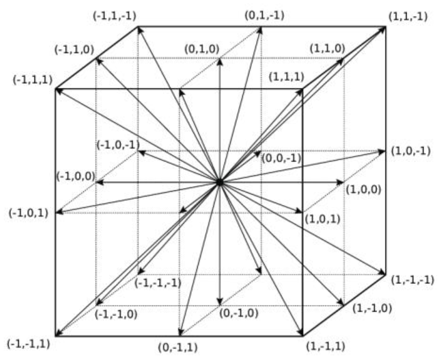
Figure 2.
XFlow octree scheme [36].
Figure 2.
XFlow octree scheme [36].
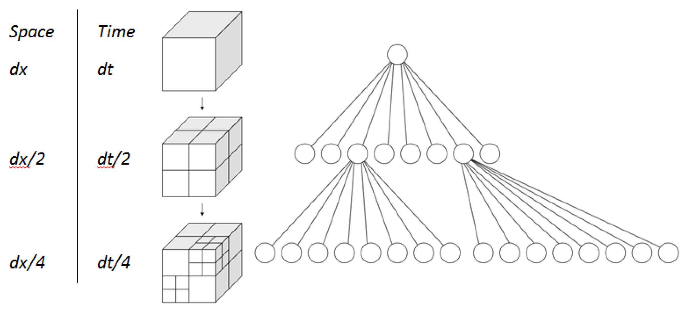
Figure 3.
3D model of the heave plate (dimensions in mm).

Figure 4.
Domains for the different symmetry cases: full domain(a), half domain (b) and quarter domain (c).
Figure 4.
Domains for the different symmetry cases: full domain(a), half domain (b) and quarter domain (c).
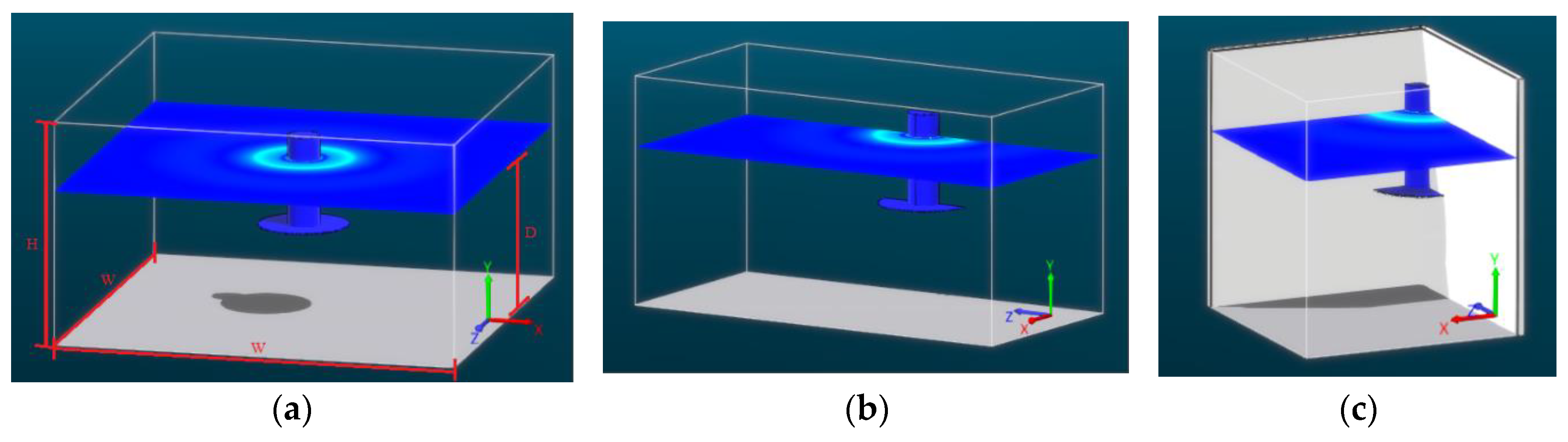
Figure 5.
Comparison between models of a similar mean error but different SNR: SNR 30.44 dB (a) and SNR 18.84 dB (b).
Figure 5.
Comparison between models of a similar mean error but different SNR: SNR 30.44 dB (a) and SNR 18.84 dB (b).
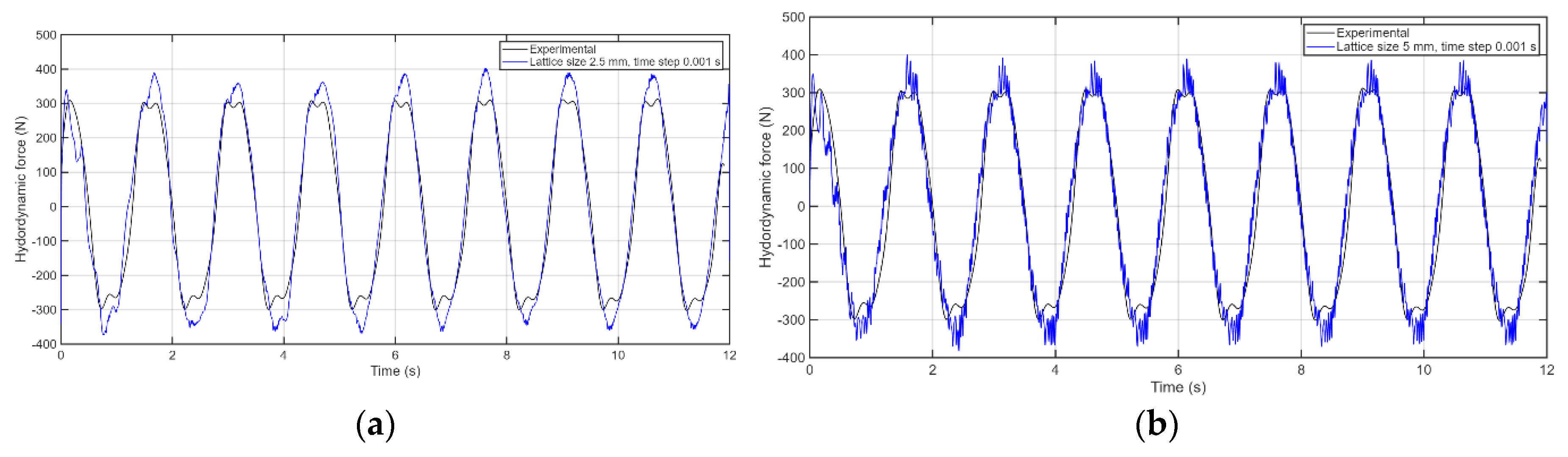
Figure 6.
Hydrodynamic force coefficients obtained for the extreme cases tested: KC=0.078 and β=1108376 (a), KC=0.078 and β=332231 (b), KC=0.754 and β=249138 (c) and KC=0.754 and β=332231 (d).
Figure 6.
Hydrodynamic force coefficients obtained for the extreme cases tested: KC=0.078 and β=1108376 (a), KC=0.078 and β=332231 (b), KC=0.754 and β=249138 (c) and KC=0.754 and β=332231 (d).
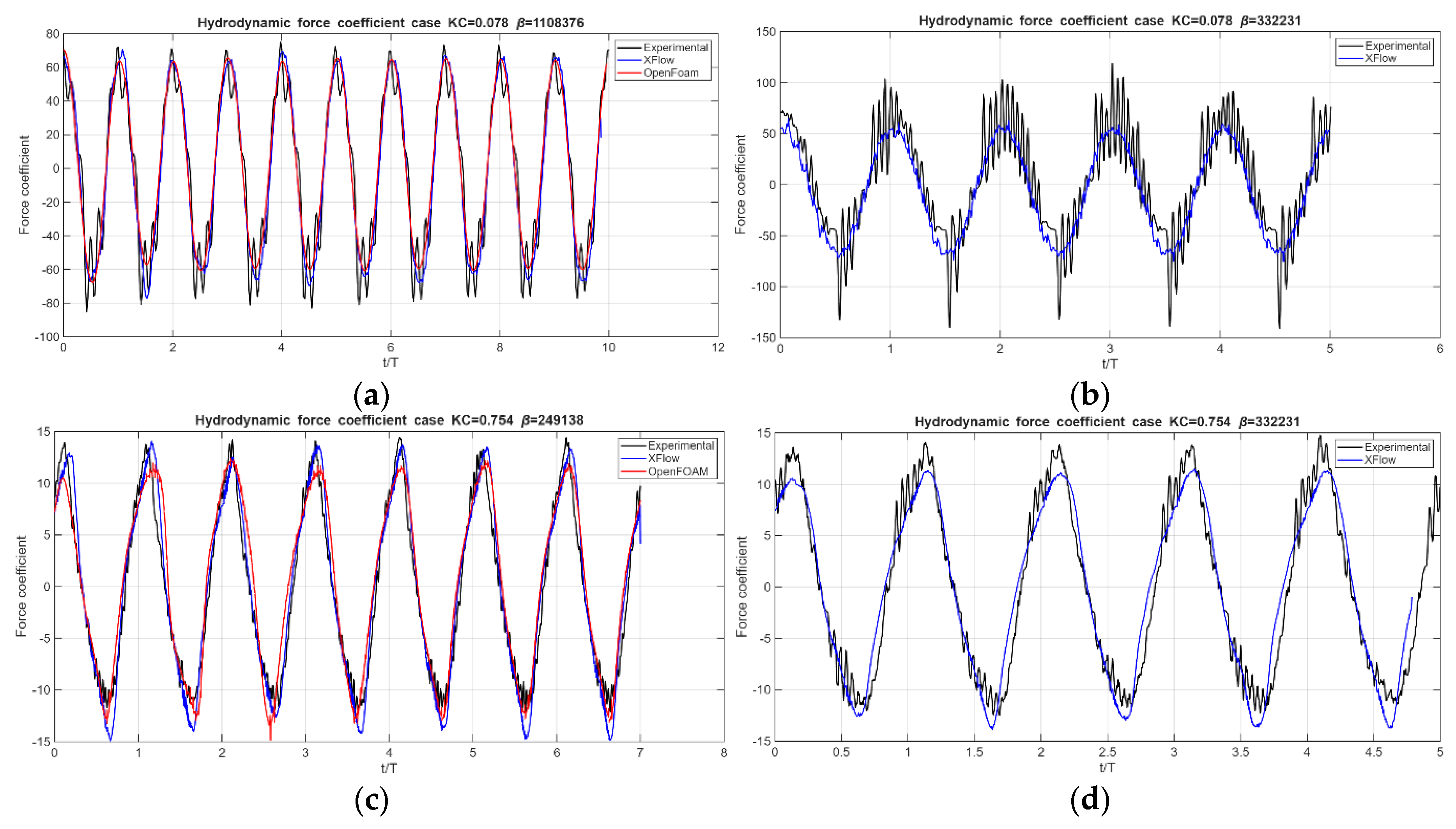
Figure 7.
Comparison of the added mass (a) and the damping (b) coefficients between the XFlow simulations, the experiments [24] and OpenFOAM simulations [35].
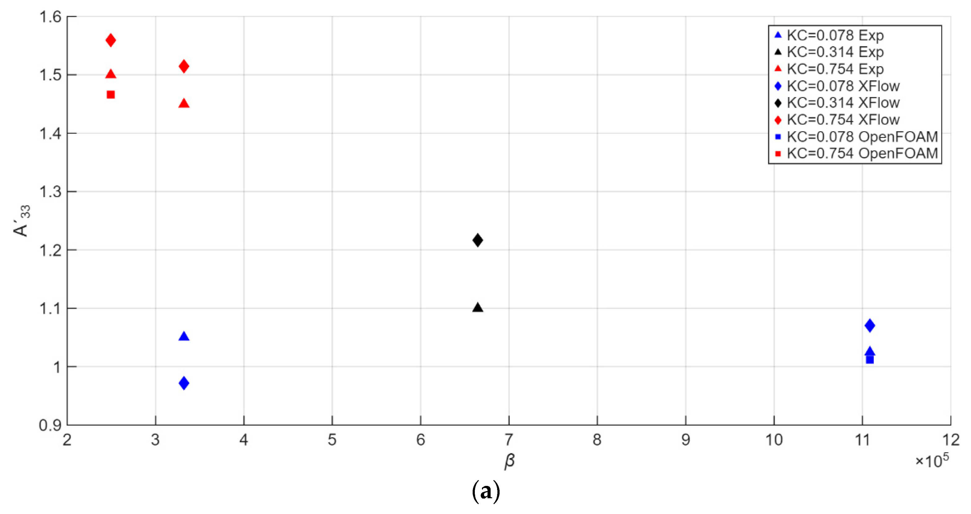
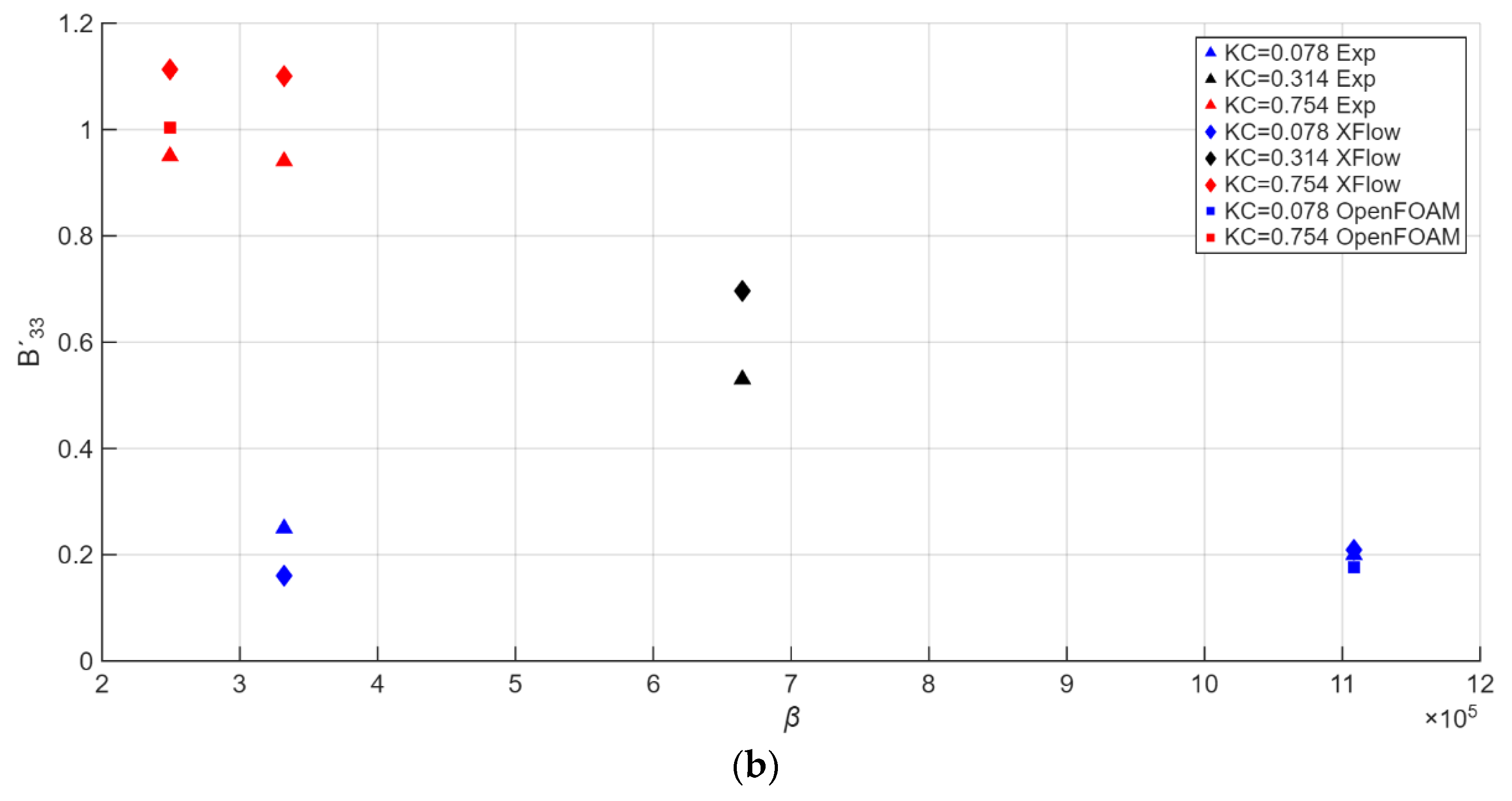
Figure 8.
Vorticity field for KC=0.078, β=1108376 (a) and KC=0.078, β=332231. (b).
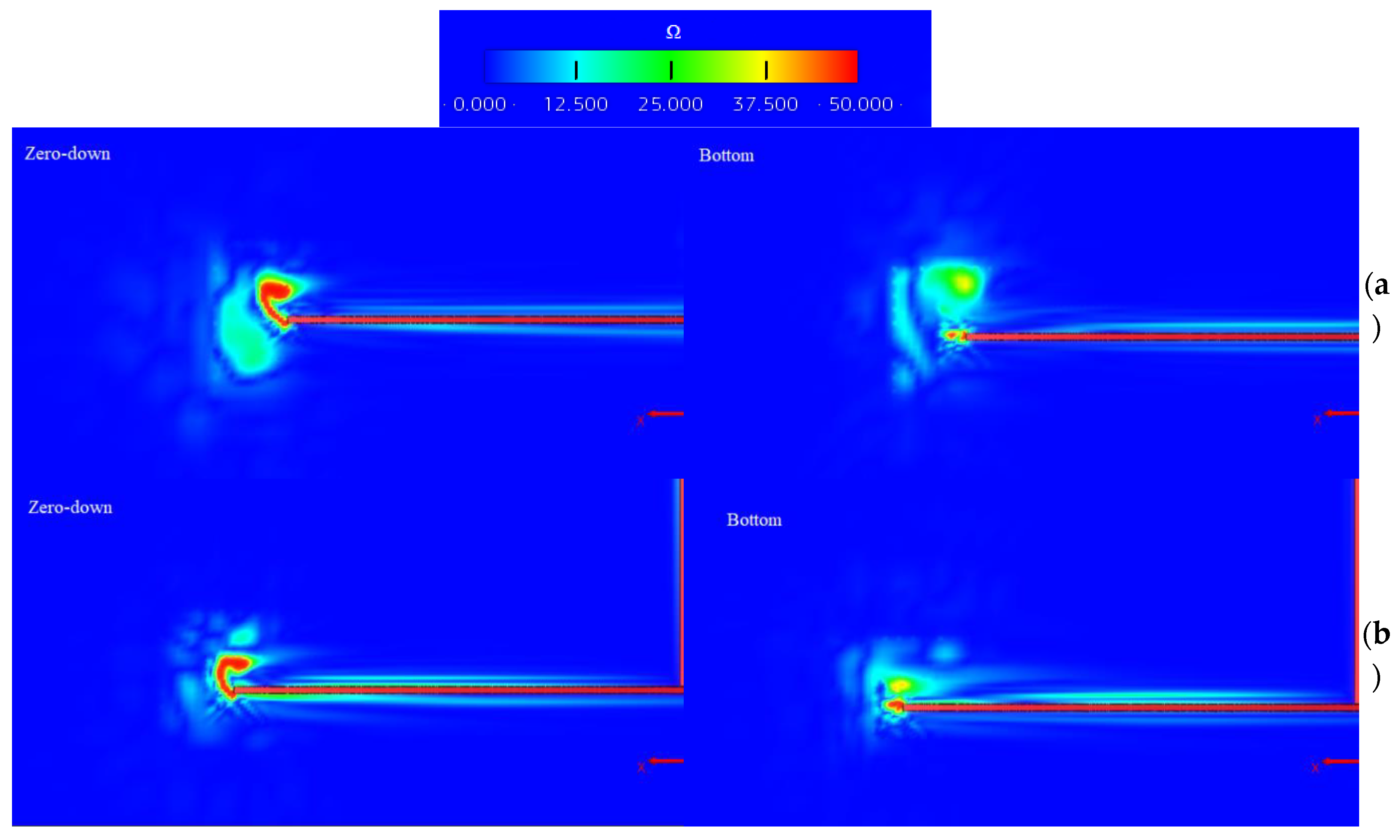
Figure 9.
Vorticity field for KC=0.754, β=332231 (a) and KC=0.754, β=249138. (b).
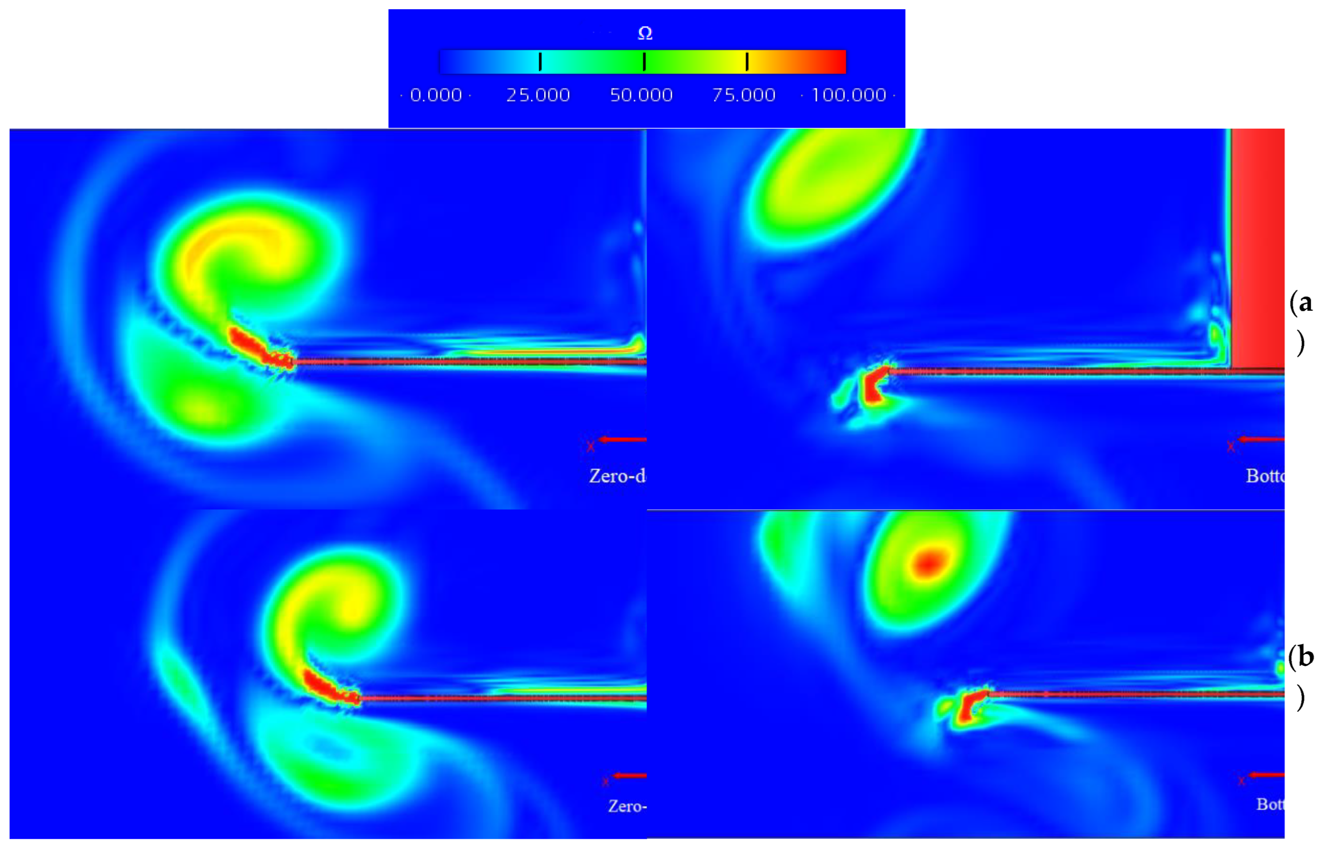
Figure 10.
Radial line (a) and cylinder (b) for pressure integration.
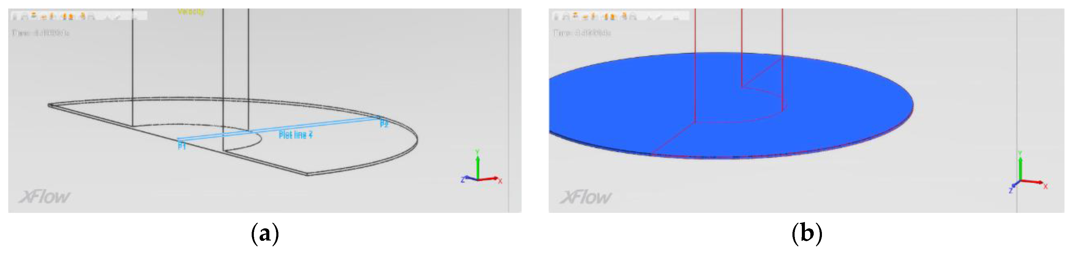
Figure 11.
Total pressure fields for the zero-downwards position (a) and bottom position (b).
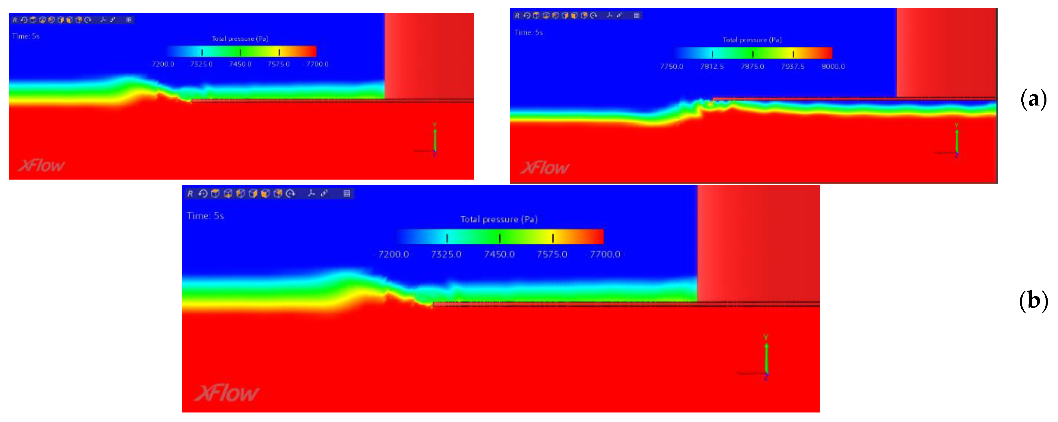

Table 1.
Summary of cases.
| Case | KC | β | A (mm) | T (s) |
|---|---|---|---|---|
| Convergence | 0.314 | 664709 | 50 | 1.5 |
| Case 1 | 0.078 | 1108376 | 12.5 | 0.9 |
| Case 2 | 0.078 | 332231 | 12.5 | 3 |
| Case 3 | 0.754 | 249138 | 120 | 4 |
| Case 4 | 0.754 | 332231 | 120 | 3 |
Table 2.
Summary of lattices and time steps.
| Lattice type | Min. size (mm) | Free surface size (mm) | Max. size (mm) |
|---|---|---|---|
| Lattice 1 | 2.5 | 5 | 10 |
| Lattice 2 | 5 | 10 | 20 |
| Time step (s) | 0.0005 | 0.001 | 0.002 |
Table 3.
Convergence study, results.
| Lattice size (mm) | Time step (s) | Cores | Computational cost (days) | Time step convergence | Mean error (%) | SNR (dB) |
|---|---|---|---|---|---|---|
| 2.5 | 0.0005 | 32 | 36 | ✓ | 12.7 | 23.63 |
| 2.5 | 0.001 | 16 | 29.9 | ✓ | 6.1 | 30.44 |
| 5 | 0.0005 | 16 | 11 | ✓ | 37 | 8.93 |
| 5 | 0.001 | 16 | 5.5 | ✓ | 5.6 | 18.84 |
Table 4.
Half and quarter symmetry study of the selected model.
| Symmetry model | Cores | Computational cost (%) | Mean error w.r.t. original model (%) | Mean error w.r.t. exp. (%) | SNR (dB) |
|---|---|---|---|---|---|
| Half | 32 | -21.4 | 4.29 | 6.7 | 32.86 |
| Quarter | 16 | -73.24 | 9.89 | 13.1 | 39.8 |
Table 5.
Convergence study for lattice size 1.67 mm with symmetry models.
| Symmetry | Min. lattice size (mm) | Time step (s) | Cores | Computational cost (days) | Mean error (%) | SNR (dB) |
|---|---|---|---|---|---|---|
| Half | 1.67 | 0.0005 | 32 | 73.1 | 13.4 | 32.11 |
| Half | 1.67 | 0.001 | 32 | 36.8 | 24.8 | 43.29 |
| Quarter | 1.67 | 0.0005 | 16 | 41.5 | 8.3 | 34.12 |
| Quarter | 1.67 | 0.001 | 32 | 12.5 | 28 | 36.86 |
Table 6.
Added mass and damping coefficients. Comparison with reference values [24].
Table 6.
Added mass and damping coefficients. Comparison with reference values [24].
| KC | β | A’33 exp. | A’33 XFlow | Difference (%) | B’33 exp. | B’33 XFlow | Difference (%) |
|---|---|---|---|---|---|---|---|
| 0.078 | 1108376 | 1.025 | 1.07 | 4.4 | 0.2 | 0.21 | 4.8 |
| 0.078 | 332231 | 1.05 | 0.97 | 7.5 | 0.25 | 0.16 | 35.6 |
| 0.754 | 249138 | 1.5 | 1.56 | 3.9 | 0.95 | 1.11 | 17.2 |
| 0.754 | 332231 | 1.45 | 1.51 | 4.2 | 0.94 | 1.1 | 17.1 |
| 0.314 | 664709 | 1.1 | 1.22 | 10.6 | 0.53 | 0.69 | 31.4 |
Table 7.
Pressure integration approaches and differences w.r.t. reference force for all cases.
| Bottom | Top | Zero-down | Zero-up | |||||||||
| Ref. (N) | Azim. (%) | Surf. (%) | Ref. (N) | Azim. (%) | Surf. (%) | Ref. (N) | Azim. (%) | Surf. (%) | Ref. (N) | Azim. (%) | Surf. (%) | |
| Case 1 | 576.3 | 0.87 | 0.47 | 957.3 | 2.57 | 1.58 | 792.5 | 2.71 | 1.17 | 722.3 | 3.10 | 1.02 |
| Case 2 | 756.2 | 2.66 | -1.31 | 767.8 | 2.66 | -1.08 | 764.6 | 3.03 | -1.18 | 759.5 | 2.92 | -1.21 |
| Case 3 | 762.4 | -17.75 | -1.24 | 745.8 | 18.19 | 8.28 | 884.1 | 23.98 | 3.45 | 677.8 | -0.66 | 5.95 |
| Case 4 | 658.8 | -4.82 | -0.72 | 844.6 | 4.37 | 5.55 | 991.7 | 10.54 | 6.76 | 623.8 | 7.94 | 5.84 |
| Conv. | 502.7 | -3.33 | -7.48 | 1025.2 | 6.33 | 3.45 | 1034.2 | -26.95 | -8.32 | 514.0 | 2.77 | -2.63 |
Disclaimer/Publisher’s Note: The statements, opinions and data contained in all publications are solely those of the individual author(s) and contributor(s) and not of MDPI and/or the editor(s). MDPI and/or the editor(s) disclaim responsibility for any injury to people or property resulting from any ideas, methods, instructions or products referred to in the content. |
© 2025 by the authors. Licensee MDPI, Basel, Switzerland. This article is an open access article distributed under the terms and conditions of the Creative Commons Attribution (CC BY) license (http://creativecommons.org/licenses/by/4.0/).
Copyright: This open access article is published under a Creative Commons CC BY 4.0 license, which permit the free download, distribution, and reuse, provided that the author and preprint are cited in any reuse.


