
Submitted:
01 December 2025
Posted:
03 December 2025
You are already at the latest version
Abstract
Wind design aims to ensure the stability, safety, and durability of a structure exposed to wind forces. Therefore, a comparative study using Computational Fluid Dynamics (CFD) was conducted to evaluate the effects of surrounding structures in wind building design. Two scenarios were analyzed: the first, in which the building was exposed to an open field, and the second, in which the building was surrounded by other buildings of equal or lower height. A CFD model, previously calibrated with experimental data, was used to simulate wind behavior. The results obtained showed significant differences between the two scenarios, confirming that nearby structures have a considerable impact on the distribution of wind pressures on the building. Therefore, the importance of considering surrounding buildings is highlighted. It is suggested that CFD can be a useful complementary tool for obtaining pressure coefficients and for the detailed analysis of wind behavior, which could improve the design and safety of buildings under wind loads.
Keywords:
CFD
; pressure coefficients
; turbulence
; velocity profile
; wind effects
; surrounding buildings
1. Introduction
In structural engineering one of the principal objectives is to make a design that guarantees the security, resilience, and durability of the structure. Is for it that all loads that can influence the structure must be considered [1], such as dead loads, live loads and the accidentals loads. The accidentals loads are those that can emerge suddenly acting during a short period of time, but their presence can harm the stability of the structure, such as effects of earthquakes, snow loads and the effects of wind [2]. Countries such as: Germany, France, United Kingdom and Mexico are severely exposed to wind action, so, there has been damage to buildings [3].
Wind is a fluid, that can produce damage on structures when they are exposed to high wind speeds, that provoke economics losses[4]. Wind effects are of high difficultly to replicate perfectly, due to vorticity effects and turbulence flows, in addition is the obtention of pressure coefficients and pressures that impact on a structure [5].For analyzing the wind effects requires experimental studies such as wind tunnel and full scale measurements, in both cases expensive tools are required in addition to carefully calibration. In wind tunnels scaled models with real fluids are studied. [6].
In order to determine wind effects over a structure, exists normative such as the Eurocode (NE-EN 1991-1-4), Normas Técnicas Complemetarias de la Ciudad de México (NTC-2023), American Society of Civil Engineers (ASCE 7), etc. In general, these codes present a methodology to estimate pressure coefficients over the surface of the structure, however, these values are constant even in the presence of surrounding structures [7].
In wind design, necessarily know the characteristics of the zone, such as the rugosity of the land. Studies demonstrate that in the urban area, the presence the other structures are high influence in the wind effects, increasing rugosity in the wind, reducing the velocity, but generating other effects such as the turbulence and vorticity[8], [9] .Analyzing an urban area, is very complicated for the effects that generates and instability of flow, is important to take into account parameters such as the burst factor, because, it relates the maximum velocity of the wind in the area and medium flow which allows evaluate the extreme conditions [10].
The urban area is increasingly big and with that, the number of high-rise buildings is growing in structural engineering. These buildings are designed to resist the high loads for winds[11]. Therefore, it is important to study the wind effects on urban areas. Currently, with advances in technology strategies have been employed for this type of study, with the implementation of software use and of mathematical models.
The CFD (Computational Fluids Dynamics), is a branch of fluid mechanics that analyzes highly complex fluid problems using mathematical models and computers, based on the laws of conservation.[12], [13], [14] .This is using for analyzing the fluids such as the wind, where studies have demonstrated, that the geometry, type of mesh, orthogonal quality, the turbulence models, solutions methods Due to the good performance of CFD in predicting wind effects [15], a series of processes based on parameters obtained from the state of the art and from the general configuration of CFD (Figure 1) were carried out in this study.
Studies have shown that the presence of surrounding structures influence in the precision of the prediction of path of wind [17]. In Table 1, a compilation of studies are shown where CFD has been used and criteria have been found to evaluate its veracity.
The CFD, in wind engineering, is used to conduct studies that analyze the effects of wind at pedestrian level, to evaluate pedestrian comfort, avoiding possible economic losses because of gusts produced[21]. Besides, studies have focused on the effects of wind on high-rise buildings, while others analyze wind behavior in the presence of vegetation and air quality in the area. However, little research has been done on the influence of surrounding buildings and how these influence the distribution of pressure coefficients over a building's surface[22].
Aim of this study was to evaluate the influence of surrounding structures on the pressure coefficients on a tall building in an urban area using CFD.
2. Materials and Methods
For this study, two scenarios were developed: the first: CFD model calibration with experimental data such as wind tunnel tests and full-scale samples, where the building is surrounded by buildings of equal or lesser height in an urban area; the second, based on the considerations of the first, shows only a completely isolated building exposed in an open field.
2.1. Scenario 1
For this case, a tall, regular building in a dense urban area surrounded by structures of equal or lesser height; therefore, the structures closest to the building of study were considered. The three phases of the CFD model used for the first scenario are described below.
2.1.1. Pre-Process
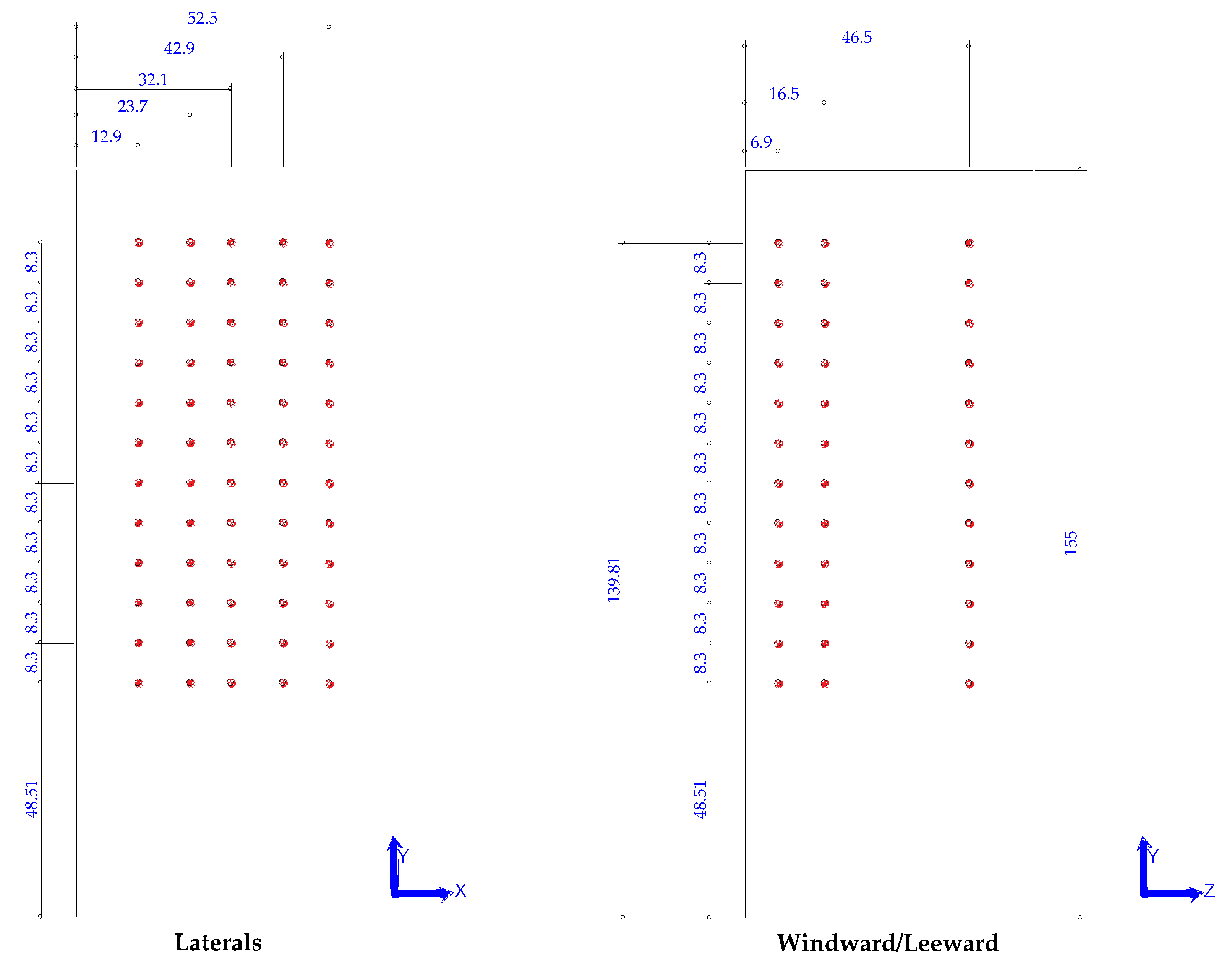
The object of study of this research is a regular-shaped high-rise building with a floor plan measuring 59.4 x 59.4 meters and a height of 155 meters (Figure 2), located in the city of Yokohama, Japan. The building is surrounded by 10 structures of equal or lower height. Data was obtained regarding its geometry and experimental studies, such as a wind tunnel and full-scale measurements were obtained from a study conducted by Kikuchi et al., [23].
To perform the geometry, which refers to a scenario in which the building under study is surrounded by other buildings, it is worth mentioning that approximate measurements were used to develop the geometry of the surrounding buildings to conduct this investigation. The floor plan measurements are shown in Figure 2.
In developing the domain, the dimensions were in relation to the size of the building (object of study), where the height is defined as H and the sides of the building, being symmetrical, are defined as L: the dimensions of the domain were established as shown in Figure 3 a), the measurements were taken from the limits of the surrounding buildings. For scenario 1, the same dimensions were considered, but the measurements were taken from the limits of the building as shown in Figure 3.
For scenario 1, where the flow inlet is in the front zone of the domain at 6L from the limits of the surrounding structures. For the side edges and the top edge, a symmetry condition was applied, indicating that the flow is continuous over those limits, as shown in Figure 4.
The meshing techniques applied for this study were validated with respect to experimental studies, where the model calibration was performed by evaluating two turbulence models, k-ε and k-ω-SST, with two different types of meshes, polyhedra and poly-hexacore with two solution methods: simple and coupled, in this process the result was that the most accurate simulation with respect to experimental studies is the configuration of a k-w-SST turbulence model. In its simple solution method with a poly-hexacore mesh because it adapts better to irregular surfaces and due to its hexacore elements, requires lower computational cost by coupling optimally to the rest of the domain. [24].
Polyhedra. The mesh size of the building was first developed, which was obtained from 10% of the building's height, that is, 1% of 155 m, resulting in a total of 1.5 m. This simplified the model and reduced the number of elements, thereby lowering the computational cost. Furthermore, it facilitated detailed coverage of the area of interest, as the mesh size was relatively small compared to the domain size [25].
A local face size was applied with respect to the building of interest, unifying the building's mesh size with a local size of 1.5 m. Additionally, a local region refinement was applied to achieve greater accuracy in data acquisition by refining the mesh around the walls of the building of interest. The final mesh size was defined as 7.75 m, at least five times the mesh size of the building of interest. For the overall mesh size, a size of 15 m was defined with a growth rate of 1.1, to avoid abrupt changes in the increase in mesh size.
For these analyses, boundary layers must be added, which generate a roughness effect on the fluid when it impacts a solid surface. The number of layers used for the study depends on verifying that the flow analyzed is turbulent by means of the Reynolds number equation (1). If the flow is not turbulent, the boundary layer requires a greater number of layers than if it is turbulent [13]. The Reynolds number is greater than 4000, indicating turbulent flow. Therefore, a thin boundary layer is required. The flow was confirmed to be turbulent, so 10 layers were assigned with a growth rate of 1.1, which corresponds to a discrete increment factor.
Where:
V: Reference velocity (m/s)
L: Impact length (m)
ν: fluid viscosity (m2/s)
The overall mesh volume was generated with a growth rate parameter of 1.1 to avoid abrupt size transitions, and an overall size of 12.2 m was assigned because the 15 m size resulted in poor mesh quality with an Orthogonal Quality of 0.01. Ultimately, with the modifications made, a mesh with an orthogonal quality of 0.45 was obtained, which corresponds to acceptable mesh quality [26].
Polyhexacore. Local sizing was applied to the building of interest, unifying the building's mesh size with a local size of 1.1 m. Subsequently, local refinement regions were added. The mesh size defined was 3 m, at least three times the building's mesh size.
For the overall mesh size, a size of 10 m was defined with a growth rate of 1.2, to avoid abrupt changes in mesh size.
The Reynolds number was checked, resulting in a value greater than 4000, indicating turbulent flow. Therefore, 10 boundary layers were assigned with a growth rate of 1.1, corresponding to a discrete increment factor, thus avoiding abrupt changes.
A total mesh size of 10 m was established with a growth rate of 1.1, because a mesh size of 15 m resulted in a poor mesh quality of 0.01. Finally, by applying an Improve Volume Mesh, a mesh with an orthogonal quality of 0.46 was obtained, which corresponds to an acceptable mesh quality. Table 2 shows the initial conditions used in this study.
An exponential wind velocity profile was used due to its simplicity of expression (equation 2) (Figure 5: incise a), since this contributes to the precision of the simulation [27].
Where:
Vz: Wind velocity to be estimated at a height Z above ground level (m).
Vref: Reference velocity (m/s)
Z: Height variation
Zref: height related to the reference speed (m)
α: roughness exponent (Table 3)
Due to the study's sensitivity, input parameters such as kinetic energy k (3) and specific dissipation rate ω (4), which relate to the atmospheric boundary layer (ABL) of wind profiles, were considered to include more realistic parameters [23].
Where:
Friction velocity
Empirical coefficient is 0.09.
Due to the sensitivity of the study, input parameters such as kinetic energy k (3) and specific dissipation rate ω (5), associated with the atmospheric boundary layer (ABL) of the wind profiles, were considered to introduce more realistic results parameters.
Where:
Friction velocity
k: Von Karman constant, is 0.4.
Z: Height variable [m].
Z0: Terrain roughness height, is 1 m.
Where:
ϵ: turbulent energy dissipation rate [m²/s³].
Empirical coefficient is 0.09.
kinetic energy.
u*ABL, Friction velocity [m/s], represents the velocity profile affected by roughness.
Where:
Friction velocity
: Reference wind velocity [m].
: Reference height [m].
: Terrain roughness height, is 1 m.
2.1.2. Solution
The solution model was a k-w-SST model, as its calibration provided a better fit for capturing the fluid effects on the surface. This refers to CFD tests performed to evaluate and calibrate the model, the results of which have not yet been published. The solution method was simple, solving the Navier-Stokes equations by coupling the fluid pressure and velocity; 1000 iterations were used, because within that range of iterations, the flow behavior becomes constant with respect to the residual graph.
2.2 Scenario 2
2.2.1. Pre-Process, Scenario 2
In the second scenario, the dimensions were established with respect to the dimensions of the building, as shown in Figure 5, in addition to considering that the building is completely exposed to the effects of the wind, without disturbances that could influence the distributions of the pressure coefficients.
To define the boundary conditions, the entrance to the front zone of the domain was at 6L with respect to the limits of the building. The sides and the top of the domain were considered with a condition of symmetry, considering that the fluid is still continuous on those edges. The bottom of the domain was established as a wall, as shown in Figure 6.
Scenario 2 the results obtained through calibration were considered, and a poly-hexacore mesh type was generated. The meshing technique that was applied was in relation to the height of the building, to obtain the mesh size on the walls of the building the criterion was set to obtain 1% of the height of the building which corresponds to 1.5 m, however to avoid deformations on the elements it was taken as a value at 0 decimal places so the final mesh size on the edge of the building was 1 m.
Local sizing was applied to the building of interest, unifying the building's mesh size with a local size of 1 m. Additionally, local region refinement was implemented to improve data acquisition accuracy by refining the mesh relative to the building's walls. The mesh size was defined as 10 m, at least 10 times the size of the building's mesh, to reduce computational costs.
For this scenario the value of the reference wind velocity with respect to the height of the building corresponds to 1.51 m/s, the viscosity of the flow corresponds to that of air with a value of 1.5x10⁻⁵ m2/s and by solving the equation it was verified that the flow is completely turbulent, so only 5 layers were used on the wall conditions with a growth rate of 1.2 to avoid sudden changes in each of the levels of the layer, the height of the first boundary layer was 0.272 m, the end of the process, an orthogonal quality of 0.5 was obtained.
2.2.2. Solution, Scenario 2
A k-ω-SST turbulence model was used, with a simple solution method, where the same variables established in Table 4 were introduced. To conclude the process, it should be mentioned that 1500 iterations were performed.
3. Results
Figure 8 shows the representation of the profiles used for the CFD model solution, a) wind speed profile, obtained from equation 2, b) dissipation frequency profile (equation 5) and the turbulent dissipation rate profile (equation 4).
Figure 7.
Profiles used for solution model CFD: a) wind speed; b) dissipation frequency, and c) turbulent energy dissipation rate.
Figure 7.
Profiles used for solution model CFD: a) wind speed; b) dissipation frequency, and c) turbulent energy dissipation rate.
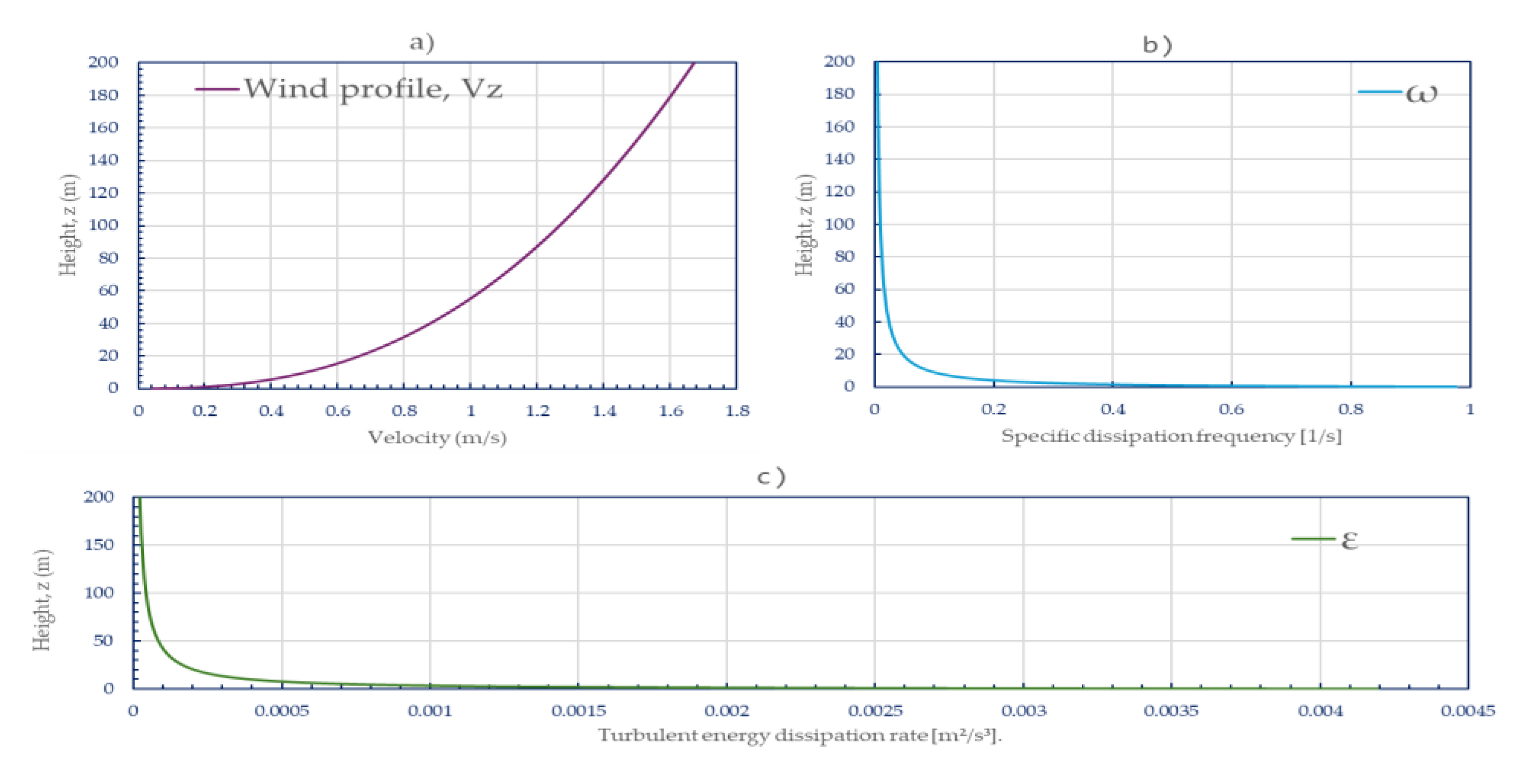
Figure 8.
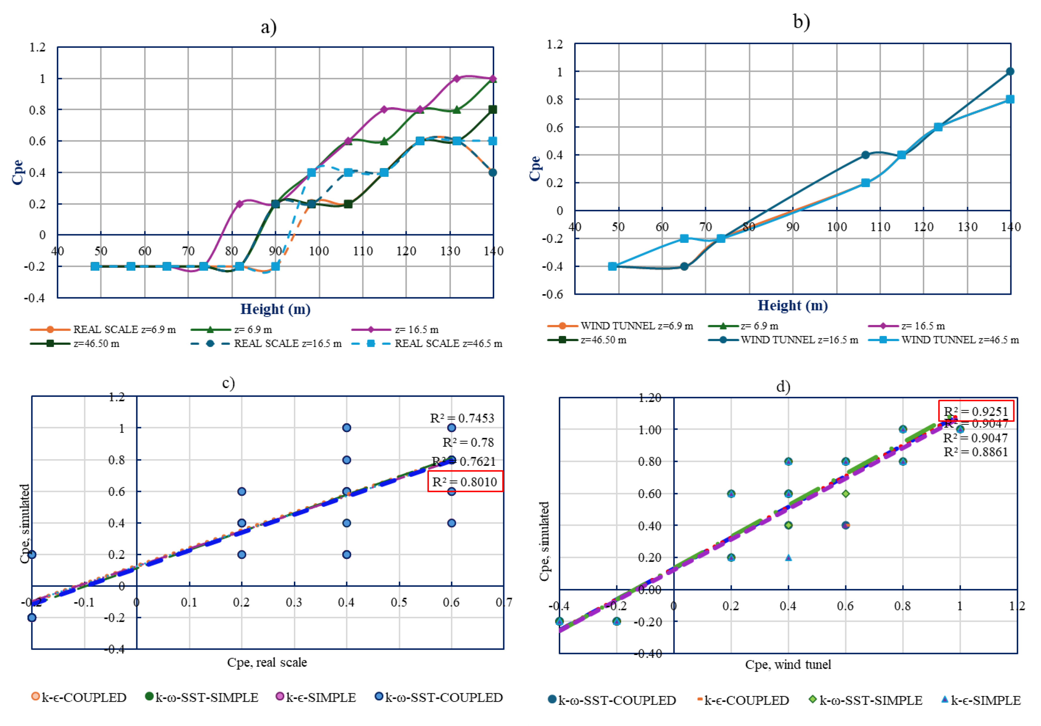
Comparison of pressure coefficients obtained from case 1 on the windward side: a) Simulated Cpe vs. Actual Scale, b) Simulated Cpe vs. Wind Tunnel, c) Linear model to determine the percentage of similarity between CFD vs. Actual Scale, and d) Linear model to determine the percentage of similarity between CFD vs. Wind Tunnel.
Figure 8.
Comparison of pressure coefficients obtained from case 1 on the windward side: a) Simulated Cpe vs. Actual Scale, b) Simulated Cpe vs. Wind Tunnel, c) Linear model to determine the percentage of similarity between CFD vs. Actual Scale, and d) Linear model to determine the percentage of similarity between CFD vs. Wind Tunnel.
3.1. Results, Scenario 1
The comparison of the CFD model, where the building is surrounded by surrounding structures that alter the wind's trajectory and cause it to directly impact the leeward side, yields result like those obtained through experimental studies, such as wind tunnels and full-scale samples. Figure 8 shows a comparison between case 1 and the experimental studies on windward. The percentage of similarity in comparisons to experimental tests is greater than 80%.
3.2. Results, Scenario 2
In case 2, where the building is located without considering the presence of surrounding structures that could influence the distribution of pressure coefficients on the building faces, as considered in current wind design regulations, the results show variability with respect to pressure coefficients compared to experimental studies.
Figure 9 shows that in section a) the results obtained by the CFD model compared to the results obtained by studies carried out on real scale, the difference in the distribution of pressure coefficients is variable, as is the case in section b) where the results are compared with pressure coefficients (Cpe) obtained by wind tunnel. This highlights the importance of considering the surrounding structures.
4. Discussion
The difference in the distribution of pressure coefficients when surrounding structures are present and when they are absent is illustrated. In a building in an open field, on a windward side, the distribution of pressure coefficients is ascending with respect to the height of the structure, and the values are positive, indicating that there is direct pressure on the building. Unlike a building surrounded by structures, the distribution changes with respect to the height of the surrounding structures and with respect to the building itself, varying the values from pressure coefficients with negative values representing suctions and positive values indicating direct pressure.
Figure 10 shows the variation of the pressure coefficients with respect to the height of the building (H) at a distance z above the face of the building.
The distribution of the values of the pressure coefficients not only varies with respect to the height of the structure, it is observed in Figure 11 that the variation is also with respect to the length of the face of the building. Furthermore, the presence of surrounding buildings not only influences the windward face, but also all four faces of the building.
In figure 11 a) it is observed that when the wind directly impacts the structure, the distribution is ascending with respect to the height of the building, and as it approaches the ends of the face of the structure, the coefficients increase. In the case where there are surrounding structures that prevent the direct impact of the wind, suction effects are generated, obtaining pressure coefficient values that vary from -0.10 in the windward case to 0.9, with a non-constant distribution, this depending entirely on the obstructions encountered.
In Figure 12, in both sections a and b, on both side faces, the distribution of pressure coefficients is similar when it comes to scenario 2. However, when there are obstructions that disturb the path of the wind, generating vortices and suctions, the distribution is variable with respect to the quantity and size of the surrounding structures. It can be seen that the behavior between both cases is different with respect to their distributions, although not so much with respect to the values.
In this case, although these are not the faces with the greatest impact from the wind, they are also significant due to the suction effects. However, it is also observed that although the case of the building exposed to open fields should generate a greater impact on the four faces of the building, the presence of the surrounding buildings does influence not only the distribution but also the obtaining of pressure coefficients on the structures.
In Figure 13(a), the similarity variation between the two models ranges from 19% to 4%, with values being more similar when the obstruction does not directly affect the structure. In the case of (b) leeward, the similarity distribution between the pressure coefficients differs considerably, ranging from 96% to 47%, highlighting the importance of surrounding structures.
The same applies to the laterals, where the coefficient of determination shows variability when comparing both cases. The relationship between the cases shows a difference of 100% to 17% for the laterals, where at a distance of 52.5 m from the x-axis, the distribution of the pressure coefficients does not coincide due to the influence of the surrounding structures.
Although the most damaging scenario for a structure designed by wind is that it is exposed to open field, through this study it is observed that the values are significantly different. In addition, some regulations for the static effects of wind on a structure consider the constant pressure coefficients on each of the faces, which generalizes the methodology but also neglects the presence of other structures, so it would also be important to carry out a study through CFD as a complementary tool for wind design in structures, although it is necessary to have adequate equipment to improve the computational cost of the simulations. Real or scale measurements of the study area should also be taken into account to have better results in terms of obtaining results.
Furthermore, although some regulations do not validate the use of CFDs for this type of studies, the Eurocode suggests CFDs as a usable tool under certain conditions.[31]
5. Conclusions
This study, using CFD simulations, confirms the importance of considering the presence of surrounding structures when analyzing wind effects, as this modifies the distribution of pressure coefficients on the building faces, resulting in an average overall reduction of 27%. Although the most unfavorable scenario is considered when a building is exposed to open terrain, this study reveals that ignoring the presence of surrounding structures would be a mistake. In open terrain, the windwards only experience positive pressure or thrust. However, the presence of surrounding structures can generate both thrust and suction on the windward side due to wind interference effects.
For future research, it is recommended to evaluate the effect of the wind's angle of incidence by varying the flow direction, as well as to analyze the influence of the location, height, and shape of surrounding buildings.
These aspects are essential, since in the present study the height, geometry and position of the target building remained constant; even so, the distribution of the pressure coefficients changed substantially due to the presence of upstream structures that obstruct and redirect the incident flow.
6. Patents
Supplementary Materials
The following supporting information can be downloaded at: https://www.mdpi.com/article/doi/s1, Figure S1: title; Table S1: title; Video S1: title.
Author Contributions
Conceptualization, C.V.-G., E.R.-G.; methodology, C.V.-G., E.R.-G.; validation, C.V.-G., E.R.-G.; formal analysis, C.V.-G., E.R.-G.; investigation, C.V.-G.; resources, C.V.-G.; data curation, C.V.-G., E.R.-G.; writing—original draft preparation, C.V.-G.; writing—review and editing, A.E.O.-T.; supervision, E.R.-G.; writing—review and editing, I.F.A.-C., L.F.P.-M. All authors have read and agreed to the published version of the manuscript.
Funding
This research did not receive external funding.
Acknowledgments
Authors would like to thank the Autonomous University of Querétaro, Faculty of Engineering, for the software resources used.
Citlali Villalobos-García is grateful to the National Council for Humanities, Sciences, and Technologies (CONAHCYT) for the scholarship grant, scholarship number 1347614.
Conflicts of Interest
The authors declare no conflicts of interest.
Appendix A
Appendix A.1
References
- Meli Piralla, Diseño estructural, 2a. Limusa, 2001.
- Ruiz y Blanco Díaz, Mecánica de Estructuras. CIMNE, 2014.
- E. E. Koks y T. Haer., «A high-resolution wind damage model for Europe», Scientific Reports, vol. 10, n.o 1, p. 6866, abr. 2020. [CrossRef]
- Z. Ouyang y S. M. J. Spence, «Performance-based wind-induced structural and envelope damage assessment of engineered buildings through nonlinear dynamic analysis», Journal of Wind Engineering and Industrial Aerodynamics, vol. 208, p. 104452, ene. 2021. [CrossRef]
- Tomás y M. Morales, «Revisión y estudio comparativo de la acción del viento sobre las estructuras empleando Eurocódigo y Código Técnico de la Edificación», Inf. constr., vol. 64, n.o 527, pp. 381-390, sep. 2012. [CrossRef]
- Y. Zhao, R. Li, L. Feng, Y. Wu, y N. Gao, «Boundary layer wind tunnel tests of outdoor airflow field around urban buildings: A review of methods and status», Renewable and Sustainable Energy Reviews, vol. 167, 2022. [En línea]. [CrossRef]
- M. Iancovici y G. B. Nica, «Time-Domain Structural Damage and Loss Estimates for Wind Loads: Road to Resilience-Targeted and Smart Buildings Design», Buildings, vol. 13, n.o 3, 2023. [CrossRef]
- Coca-Obdulio, «DAÑOS DEL VIENTO EN ZONAS URBANAS», Arquitectura y Urbanismo, vol. 29, n.o 0258-591X, pp. 64-67, 2008.
- C. Bustamante, M. Jans, y E. Higueras, «El comportamiento del viento en la morfología urbana y su incidencia en el uso estancial del espacio público, Punta Arenas, Chile», AUS, n.o 15, pp. 28-33, 2014.
- C. Lin, R. Ooka, Y. Takakuwa, y H. Kikumoto, «Wind tunnel study of Parapet effects on rooftop wind environment with implications for safe urban-air-mobility operations», Building and Environment, vol. 284, p. 113509, oct. 2025. [CrossRef]
- Ishida, Y., Yoshida, A., Yamane, Y., y Akashi Mochida, «Impact of a single high-rise building on the wind pressure acting on the surrounding low-rise buildings», Journal of Wind Engineering and Industrial Aerodynamics, vol. 250, n.o 105742, 2024. [En línea]. [CrossRef]
- Xamán, Dinámica De Fluidos Computacional Para Ingenieros. Palibrio, 2016.
- F. M. White, Mecánica de fluidos. Madrid: Mcgraw-Hill, 2010.
- H. K. Versteeg y W. Malalasekera, An Introduction to Computational Fluid Dynamics: The Finite Volume Method, Second Edition. Pearson Education Limited, 2007.
- Baghaei Daemei, E. M. Khotbehsara, E. M. Nobarani, y P. Bahrami, «Study on wind aerodynamic and flow characteristics of triangular-shaped tall buildings and CFD simulation in order to assess drag coefficient», Ain Shams Engineering Journal, vol. 10, n.o 3, pp. 541-548, sep. 2019. [CrossRef]
- Khalil y I. Lakkis, Computational Fluid Dynamics: An Introduction to Modeling and Applications, 1st Edition. McGrawHill, 2023. [En línea]. https://books.google.com.mx/books/about/Computational_Fluid_Dynamics_An_Introduc.html?id=eMCqEAAAQBAJ&redir_esc=y.
- K. Wijesooriya, D. Mohotti, C.-K. Lee, y P. Mendis, «A technical review of computational fluid dynamics (CFD) applications on wind design of tall buildings and structures: Past, present and future», Journal of Building Engineering, vol. 74, p. 106828, sep. 2023. [CrossRef]
- Z. Cheng, J. K. Wong, y O. Mercan, «Evaluating the wind loads on high-rise buildings of various plan dimensions through numerical simulations», Engineering Structures, vol. 343, n.o 120981, 2025. [En línea]. [CrossRef]
- Haan F. L., Wang J., Sterling M., y Kopp G. A., «Experimentally estimating wind load coefficients for tornadoes – An alternative perspective», Journal of Wind Engineering and Industrial AerodynamicsJournal of Wind Engineering and Industrial Aerodynamics, vol. 251, n.o 105811, 2024. [En línea]. [CrossRef]
- Idrissi, H. El Mghari, y R. El Amraoui, «CFD simulation advances in urban aerodynamics: Accuracy, validation, and high-rise building applications», Results in Engineering, vol. 26, n.o 105148, 2025. [En línea]. [CrossRef]
- F. Liu, Y. Ren, L. Zhang, y X. Li, «Impact of super high-rise buildings on wind comfort and safety of pedestrian wind environment: A case study in Shanghai, China», Case Studies in Thermal Engineering, vol. 71, p. 106197, jul. 2025. [CrossRef]
- L. Pardo-del Viejo y S. Fernández-Rodríguez, «CFD with LIDAR applied to buildings and vegetation for environmental construction», Automation in Construction, vol. 167, p. 105710, nov. 2024. [CrossRef]
- T. Kikuchi et al., «Comparison of wind pressure coefficients between wind tunnel experiments and full-scale measurements using operational data from an urban high-rise building», Building and Environment, vol. 252, p. 111244, mar. 2024. [CrossRef]
- ANSYS, Inc, «Capítulo 4: Turbulencia», Ansys Fluent R2 2024. Accedido: 13 de enero de 2025. [En línea]. https://ansyshelp.ansys.com/public/account/secured?returnurl=/Views/Secured/corp/v242/en/flu_th/flu_th_sec_turb_kw_sst.html.
- M. Fernández, Técnicas numéricas en ingeniería de fluidos : introducción a la dinámica de fluidos computacional (CFD) por el método de volúmenes finitos. Barcelona: Reverté, 2012.
- N. Fatchurrohman y S. T. Chia, «Performance of hybrid nano-micro reinforced mg metal matrix composites brake calliper: simulation approach», IOP Conference Series: Materials Science and Engineering, vol. 257, p. 012060, 2017.
- «Numerical evaluation of wind effects on a tall steel building by CFD (2007).».
- J. M. Guevara Díaz, «Cuantificación del perfil del viento hasta 100 m de altura desde la superficie y su incidencia en la climatología eólica», Terra Nueva Etapa, vol. 29, n.o 46, pp. 81-101, 2013.
- Kubilay, A. Rubin, D. Derome, y J. Carmeliet, «Wind-comfort assessment in cities undergoing densification with high-rise buildings remediated by urban trees», Journal of Wind Engineering and Industrial Aerodynamics, vol. 249, p. 105721, jun. 2024. [CrossRef]
- «CFD simulation of wind-induced pressure coefficients on buildings with and without balconies.pdf».
- European Committee for Standardization (CEN), Eurocode 1: Actions on structures — Part 1-4: General actions — Wind actions. 2005.
Figure 1.
General methodology of CFD. [16].
Figure 1.
General methodology of CFD. [16].
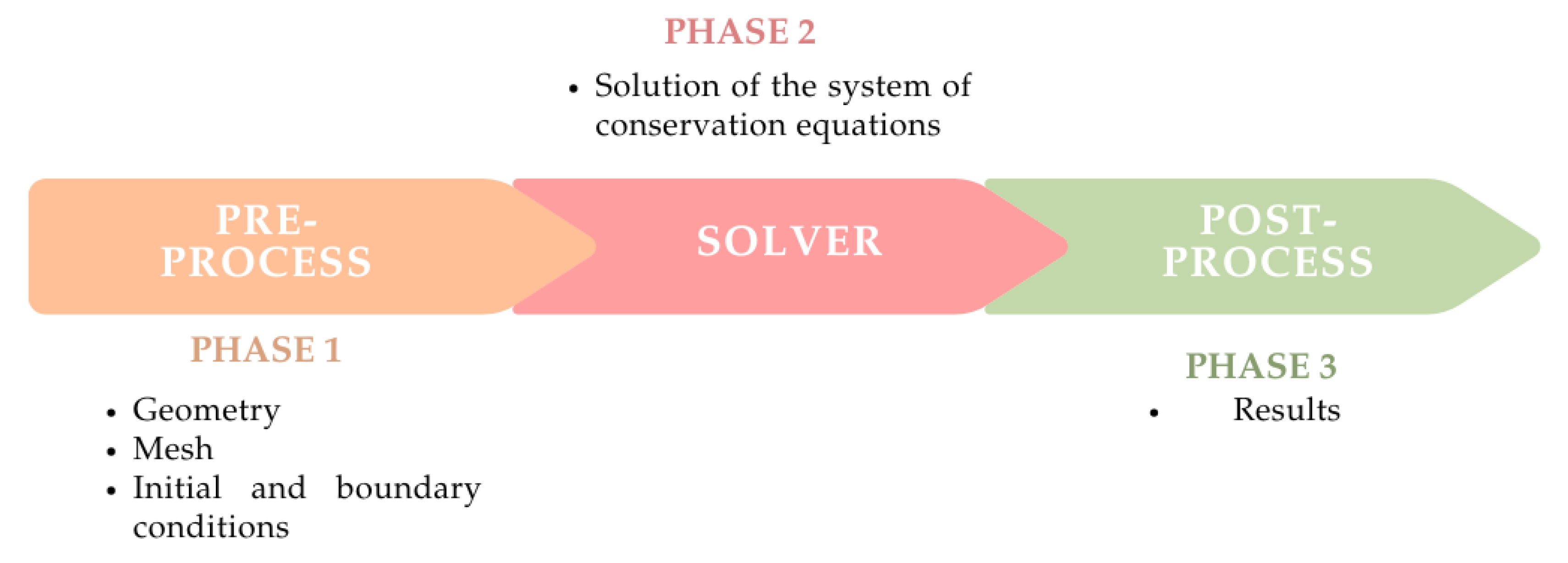
Figure 2.
Dimension of building [23].
Figure 2.
Dimension of building [23].
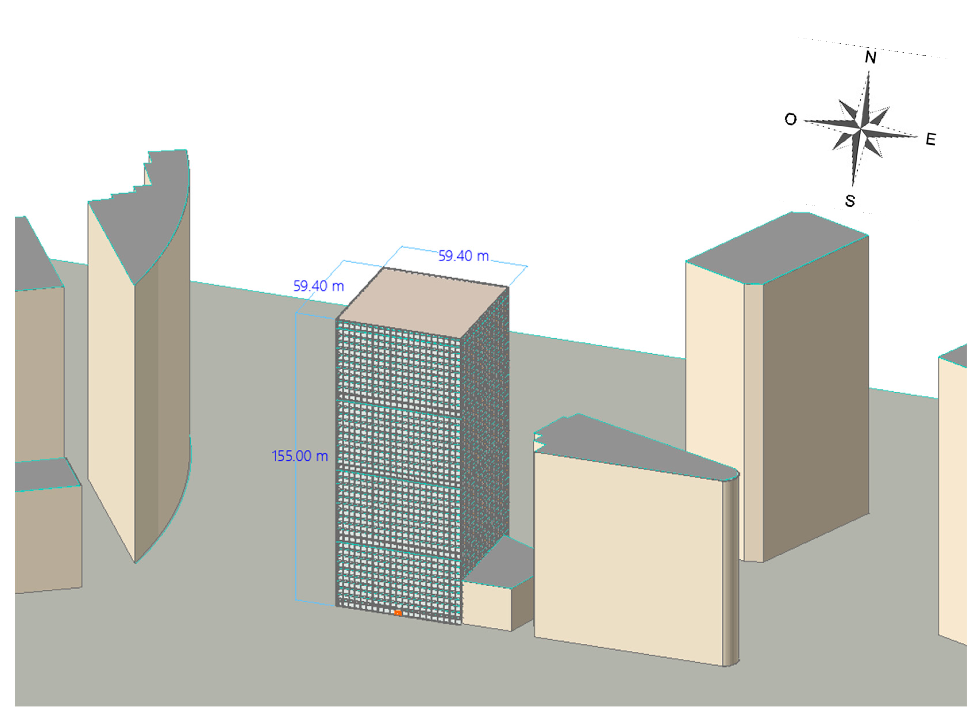
Figure 3.
Domain dimensions of scenario 1, building with surrounding structures: H: 155 m (building height), L:54.9 m (building sections) [24], modified.
Figure 3.
Domain dimensions of scenario 1, building with surrounding structures: H: 155 m (building height), L:54.9 m (building sections) [24], modified.
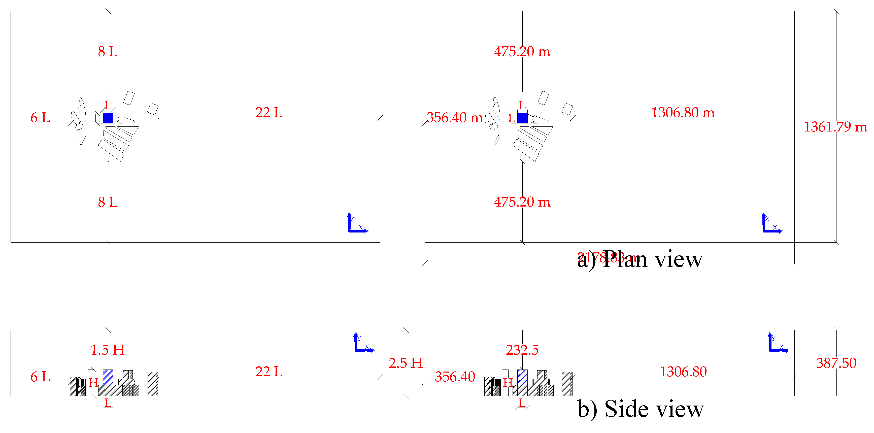
Figure 4.
Boundary conditions and domain dimensions of scenario 1.
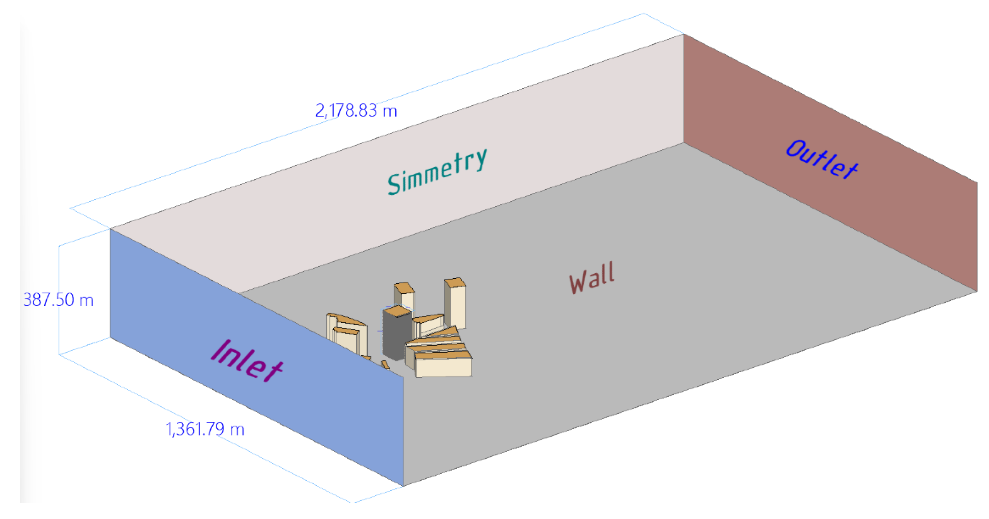
Figure 5.
Domain dimensions of case 2, open field building: H: 155 m (building height), L:54.9 m (building sections) [24], modified.
Figure 5.
Domain dimensions of case 2, open field building: H: 155 m (building height), L:54.9 m (building sections) [24], modified.
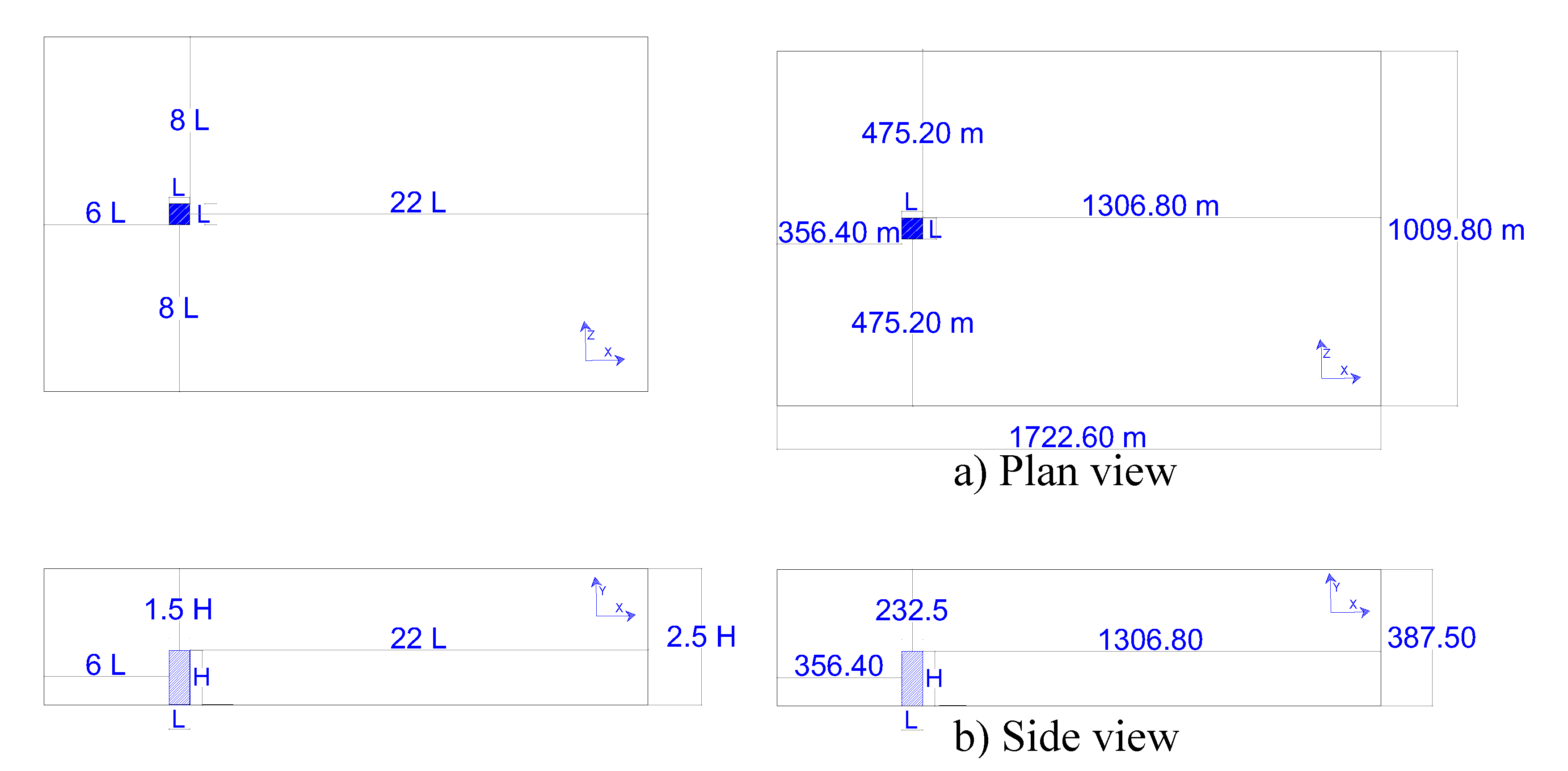
Figure 6.
boundary conditions: case 2, building exposed to open countryside.
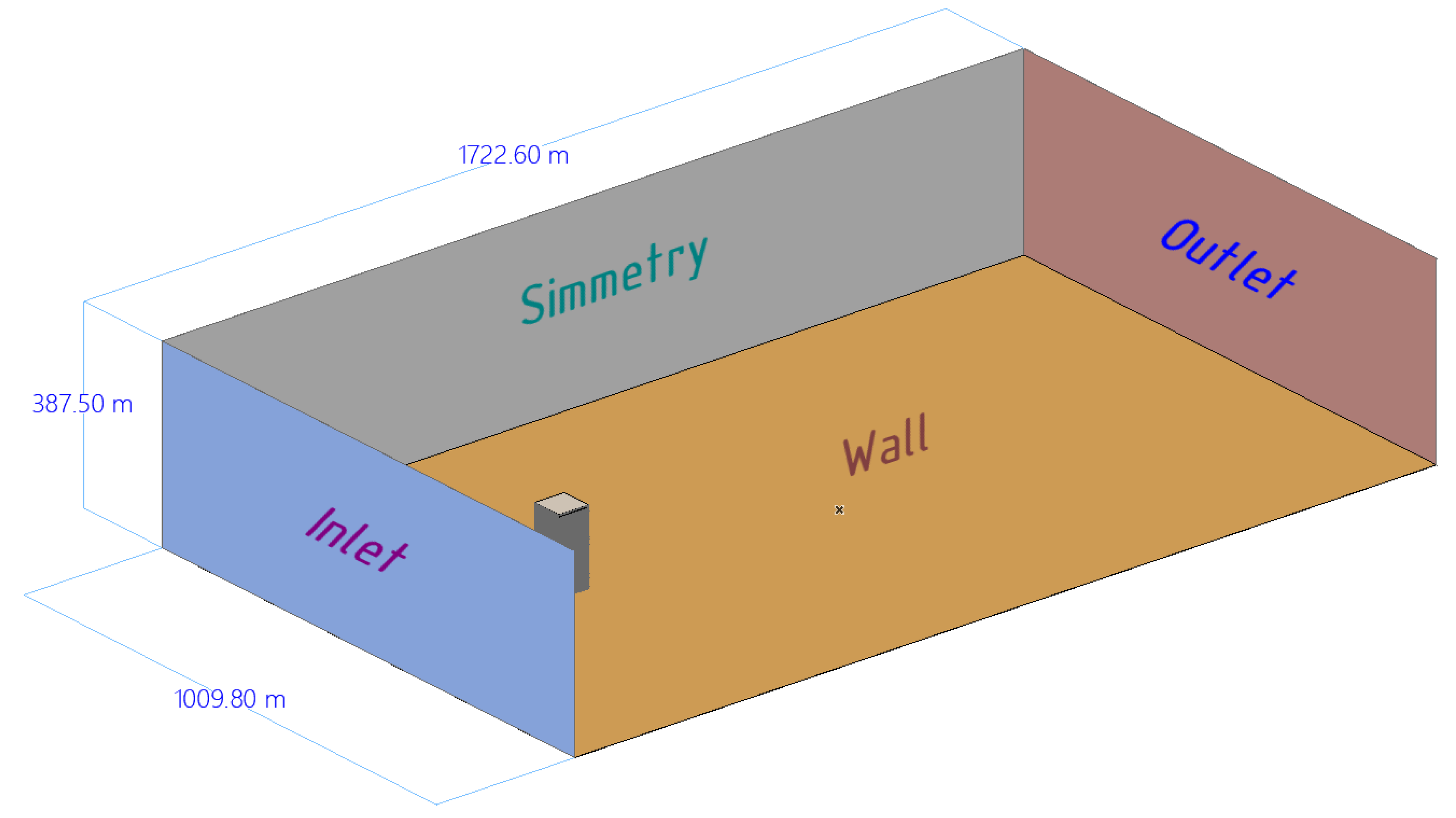
Figure 9.
Comparison of pressure coefficients obtained from case 2 on the windward side: a) Simulated Cpe vs. Actual Scale, b) Simulated Cpe vs. Wind Tunnel.
Figure 9.
Comparison of pressure coefficients obtained from case 2 on the windward side: a) Simulated Cpe vs. Actual Scale, b) Simulated Cpe vs. Wind Tunnel.
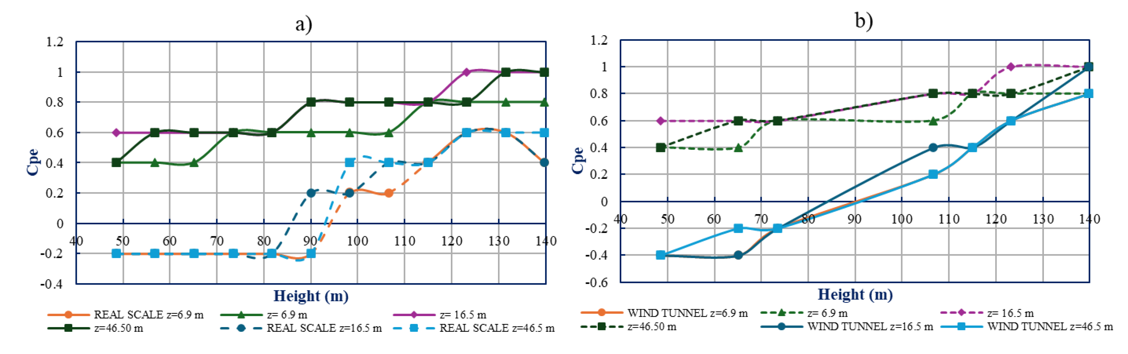
Figure 10.
Distribution of pressure coefficients with respect to height.
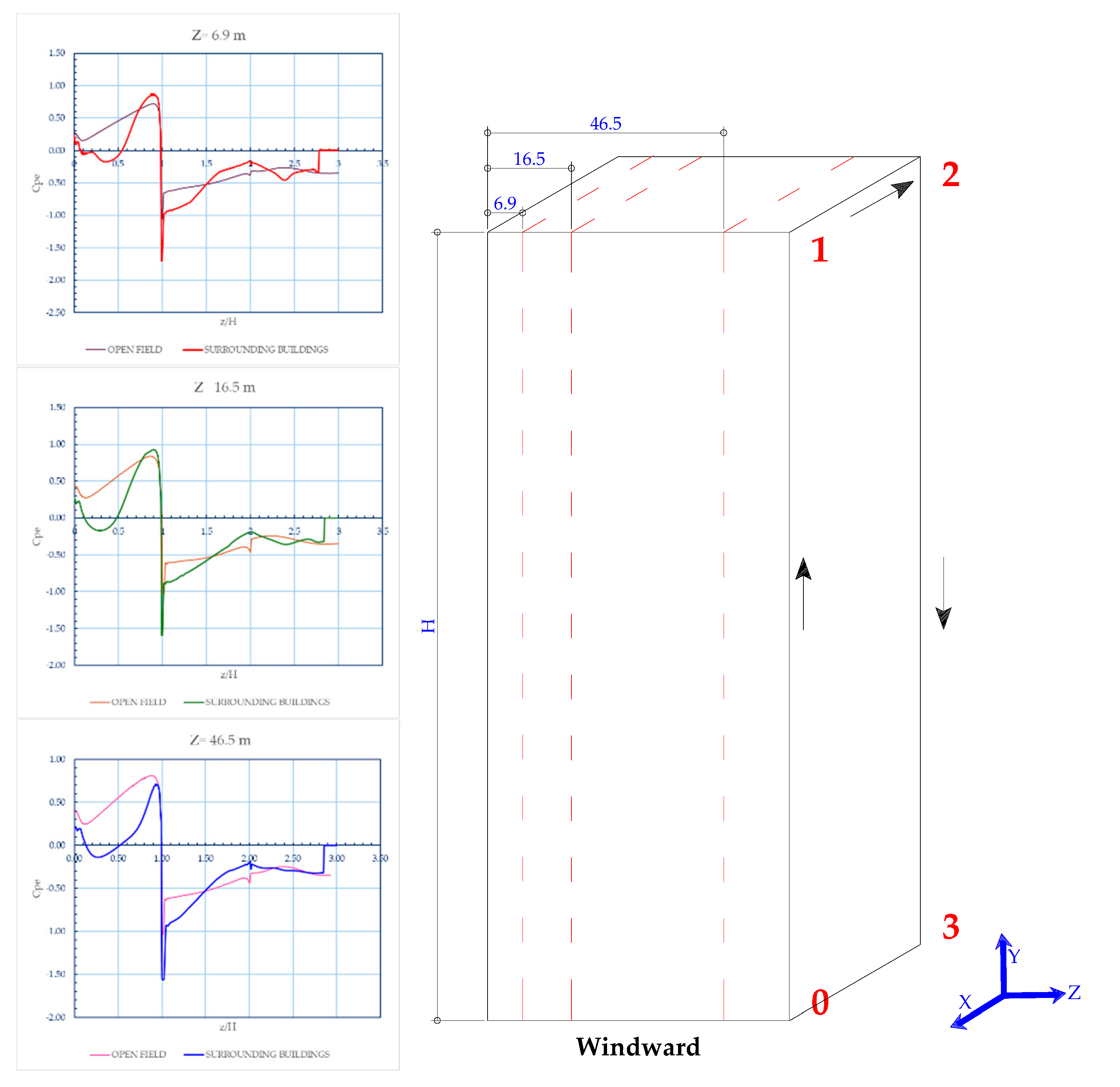
Figure 11.
Distribution of pressure coefficients when the building is located in an open field and when it is surrounded by structures of equal or lower height: a) Windward, b) Leeward.
Figure 11.
Distribution of pressure coefficients when the building is located in an open field and when it is surrounded by structures of equal or lower height: a) Windward, b) Leeward.
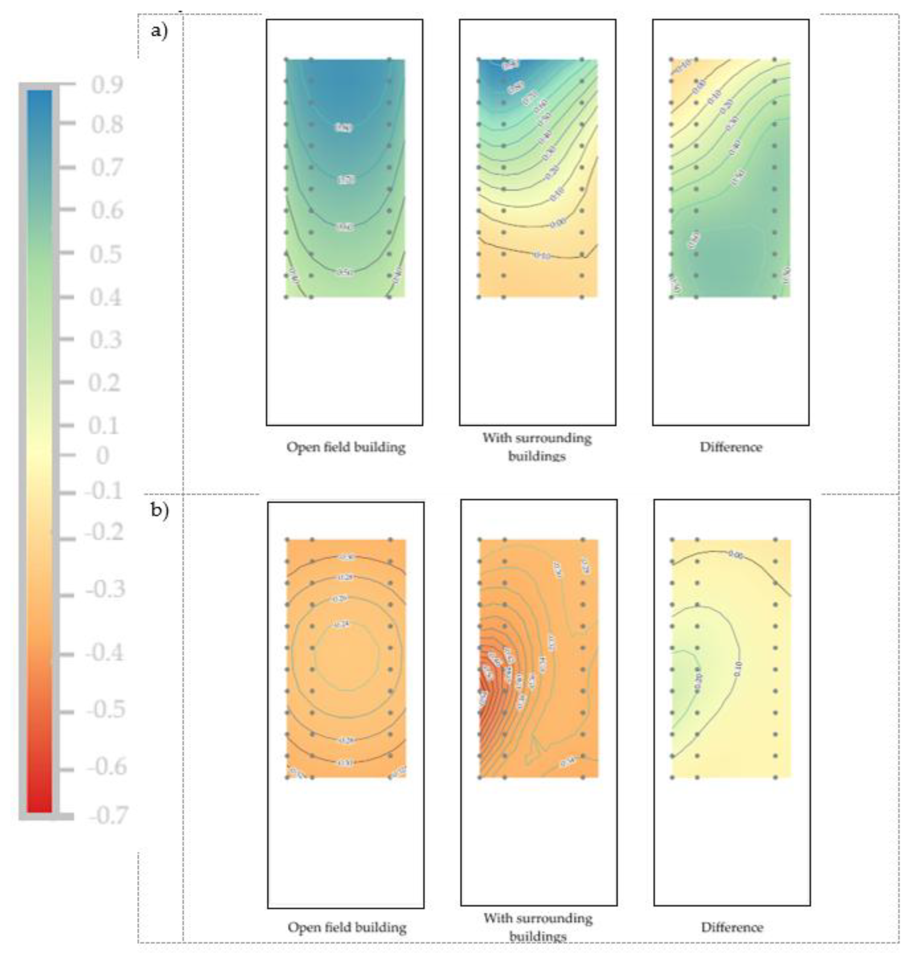
Figure 12.
Distribution of pressure coefficients on the lateral faces when the building is located in the open field and when it is surrounded by structures of equal or lower height: a) Lateral 1, northbound, b) Lateral 2, southbound.
Figure 12.
Distribution of pressure coefficients on the lateral faces when the building is located in the open field and when it is surrounded by structures of equal or lower height: a) Lateral 1, northbound, b) Lateral 2, southbound.
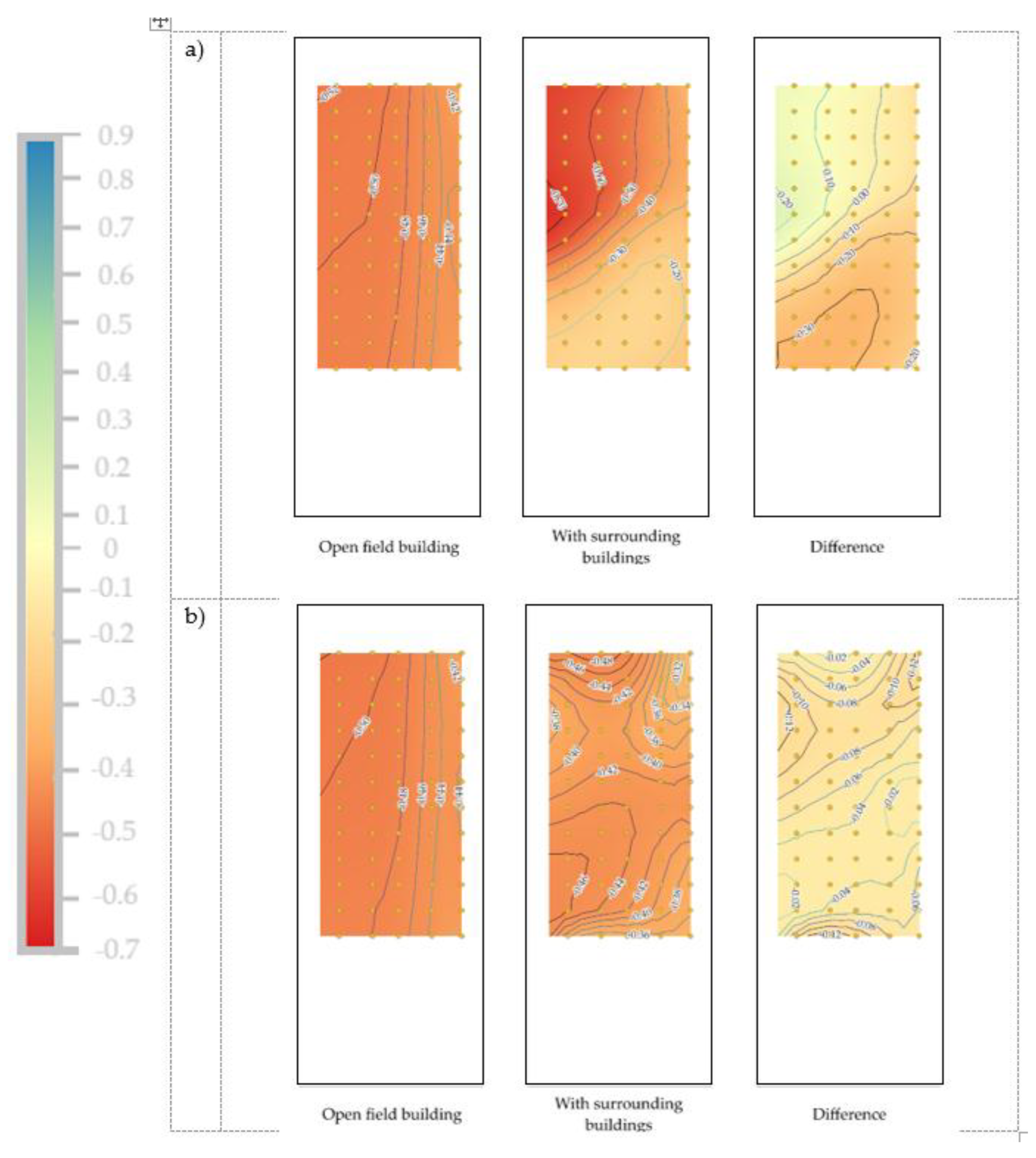
Figure 13.
Linear model to obtain the percentage of simultaneity between both cases by means of the coefficient of determination (R2) in the 4 sides of the building: a) windward, b) leeward, c) Side 1 and d) Side 2.
Figure 13.
Linear model to obtain the percentage of simultaneity between both cases by means of the coefficient of determination (R2) in the 4 sides of the building: a) windward, b) leeward, c) Side 1 and d) Side 2.
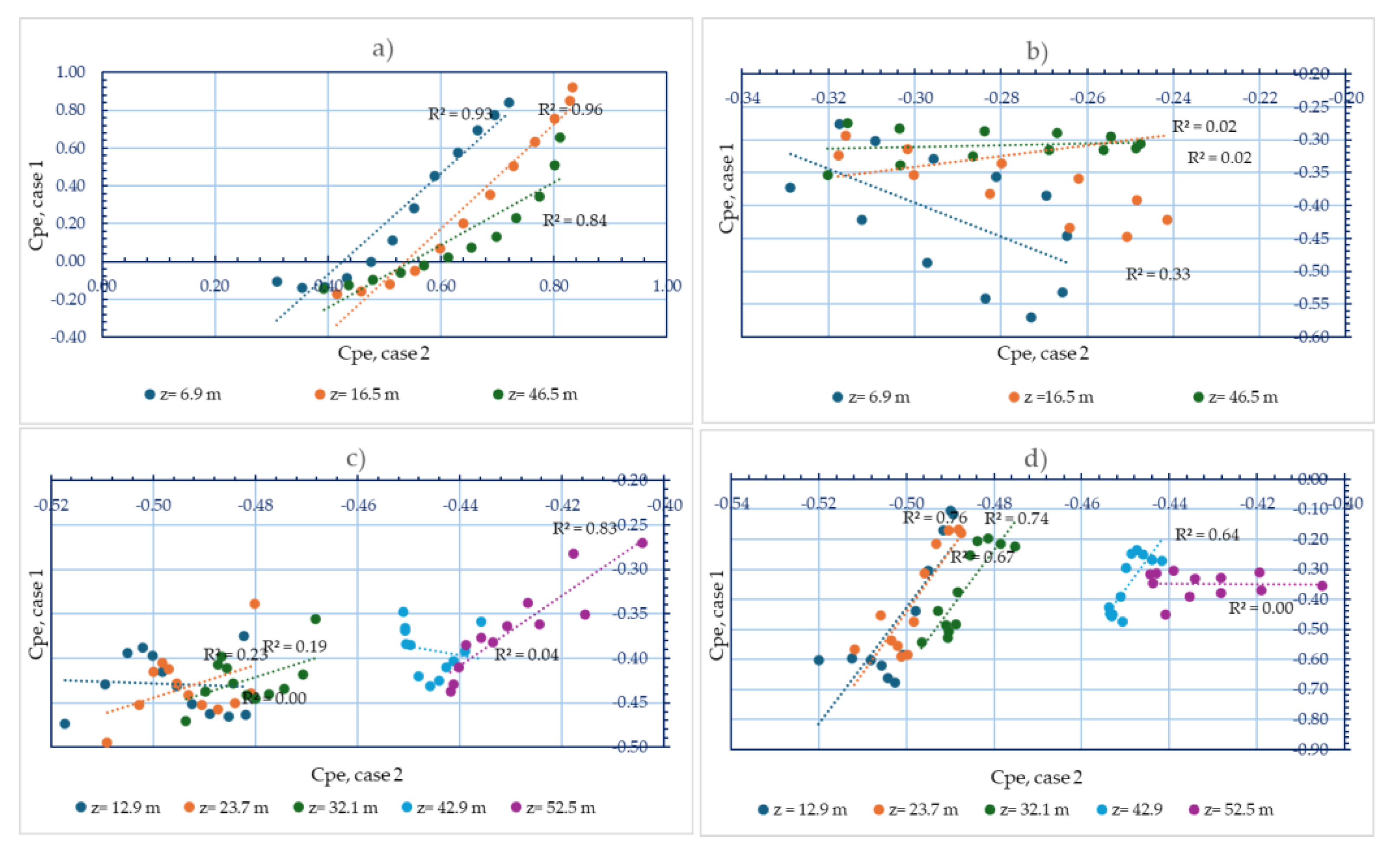

Table 1.
Collection of studies by means of state of art.
| Title | Comment | Ref |
| Evaluating the wind loads on high-rise buildings of various plan dimensions through numerical simulations. |
Checks the functionality of CFD in de capture of pressure coefficients high-rise buildings by simulations WMLES, are more precise than models RANS. |
[18] |
| Experimentally estimating wind load coefficients for tornadoes – An alternative perspective. |
Explain the importance of turbulence, and what is the relation with the applied loads on a sur-face or structure. |
[19] |
| A technical review of computational fluid dynamics (CFD) applications on wind design of tall buildings and structures: Past, present and future | Parameters such as velocity profile, mean pressure turbulence intensity profile, turbulence model and solution method influence the pressure for obtaining pressure coefficients on a surface. The LES model is more accurate than RANS but requires higher computational costs. |
[17] |
| CFD simulation advances in urban aerodynamics: Accuracy, validation, and high-rise building applications | Turbulence models such as k-ε-RNG and SST-ω-Standard were compared, including parameters like kinetic energy and the dissipation rate. To validate this research, wind tunnels studies were used. The result was that both models are reliable, but the k-ε model requires lower computational cost. | [20] |
Table 2.
Initial conditions used for solution preparation in each turbulence model.
| Parameter | value |
| Inlet velocity | 1.51 m/s |
| Outlet pressure | 0 Pa |
| Wall | No-slip |
| Air density | 1.255 kg/m3 |
| Air viscosity | 1.5x10⁻⁵ m2/s |
Table 3.
Roughness exponent values [28].
Table 3.
Roughness exponent values [28].
| Parameter | value |
| Water | 0.13 |
| Grass | 0.14-0.16 |
| Crops and shrubs | 0.20 |
| Forests | 0.25 |
| Urban area | 0.40 |
Table 4.
Input conditions and variables.
| Parameter | value |
| Inlet velocity | 1.51 m/s |
| Outlet pressure | 0 Pa |
| Wall | No-slip |
| Air density | 1.255 kg/m3 |
| Air viscosity | 1.5x10⁻⁵ m2/s |
| Wind velocity | (equation 2) |
| Kinetic energy | (equation 3) |
| Turbulent energy dissipation rate | (equation 4) |
| Specific dissipation frequency | (equation 5) |
| Friction velocity | (equation 6) |
Disclaimer/Publisher’s Note: The statements, opinions and data contained in all publications are solely those of the individual author(s) and contributor(s) and not of MDPI and/or the editor(s). MDPI and/or the editor(s) disclaim responsibility for any injury to people or property resulting from any ideas, methods, instructions or products referred to in the content. |
© 2025 by the authors. Licensee MDPI, Basel, Switzerland. This article is an open access article distributed under the terms and conditions of the Creative Commons Attribution (CC BY) license (http://creativecommons.org/licenses/by/4.0/).
Copyright: This open access article is published under a Creative Commons CC BY 4.0 license, which permit the free download, distribution, and reuse, provided that the author and preprint are cited in any reuse.


