
Submitted:
02 December 2025
Posted:
02 December 2025
You are already at the latest version
Abstract
The thermal influence of Urban Heat Islands (UHIs) is not limited to periods of high temperature but persists throughout the year. The present study utilises hourly data collected over a period of one year from a network of hygrothermal monitoring stations with a high density, which were deployed across the city of Cáceres (Spain). The network was designed in accordance with the World Meteorological Organization's guidelines for urban measurements (employing radiation footprints and surface roughness) and ensures representation of each Local Climate Zone (LCZ), characterised by those factors (such as building typology and density, urban fabric, vegetation, and anthropogenic activity, among others) that influence potential solar radiation absorption. The magnitude of the heat island effect in this city has been determined to be approximately 7 °C in summer and winter at the first hours of the morning. In order to assess the energy impact of UHIs, Cooling and Heating Degree Days (CDD & HDD) were calculated for both summer and winter periods across the different LCZs. Following the implementation of rigorous quality control procedures and the utilisation of gap-filling techniques, the analysis yielded discrepancies in energy demand of up to 10% between LCZs within the city. The significance of incorporating UHIs into the design of building envelopes and climate control systems is underscored by these findings, with the potential to enhance both energy efficiency and occupant thermal comfort. This meth-odology is particularly relevant for extrapolation to larger and denser urban environments, where the intensification of UHI effects exerts a direct impact on energy consumption and costs. The following essay will provide a comprehensive overview of the relevant literature on the subject.

Keywords:
urban heat island
; local climate zones
; urban building energy
; building energy analysis
; thermal energy demand
; heating and cooling degree days
; hygrothermal sensor network
; sustainable and resilient cities
; smart cities
1. Introduction
Contemporary cities face significant challenges arising from climate change, urban growth and increased energy demand. The need to reduce greenhouse gas emissions and improve energy efficiency has driven the development of international policies and standards aimed at a more sustainable and less risky urban model [1]. In this context, international standards such as Standard 100-2024 [2], defined by the American Society of Heating, Refrigerating and Air-Conditioning Engineers (ASHRAE), establish criteria for the assessment, auditing and improvement of energy performance in existing buildings, contributing to increasing their efficiency and resilience to climate change. Likewise, the European Union has established an ambitious regulatory framework for energy efficiency, with the aim of promoting consumption reduction and achieving a nearly zero-emission building stock by 2050 [3,4].
The construction industry in Europe is characterized by a variety of building traditions, each of which reflects not only distinct climatic and cultural conditions but also unique regulatory frameworks. These regulatory approaches significantly influence the design of buildings, thereby affecting their energy performance. In the Scandinavian context, regulatory frameworks in Finland and Sweden delineate energy efficiency targets, technical design requirements, energy management strategies, and thermal comfort criteria, emphasizing the necessity of high-quality building envelopes, thermal insulation, and the integration of renewable energy sources [5,6]. In the Anglo-Saxon region, the United Kingdom has adopted a comprehensive approach to energy measurement and monitoring, encompassing both on-site testing (blower door test) and energy simulations [7]. In Central Europe, countries such as Germany [8], Austria [9], Switzerland [10], and the Netherlands [11] have adopted specific building standards that prioritize energy efficiency and environmental sustainability. These standards include the requirement for compact, airtight buildings, the implementation of mechanical ventilation with heat recovery, and the design of buildings according to the "Passivhaus" or "Effizienzhaus" standards.
Mediterranean countries, including Italy [12], Greece [13], and Portugal [14], have established regulatory frameworks that mandate limits on thermal transmittance, solar control, and ventilation requirements, minimum efficiency levels for thermal systems, and energy demand (Heating, Ventilation and Air Conditioning (HVAC) and domestic hot water). These regulatory measures promote the development of nearly zero-energy buildings (nZEB), emphasizing the integration of energy efficiency and sustainability. France, situated in an intermediate position between Central Europe and the Mediterranean, exhibits a combination of characteristics indicative of both regions. On the one hand, it displays the high-quality envelopes and airtightness characteristic of Central European countries. On the other hand, it exhibits solar control and overheating protection strategies through passive design, characteristics of Mediterranean countries [15].
In the specific case of Spain, which belongs to the Mediterranean zone and is the focus of this paper, the design criteria for buildings in terms of energy efficiency are primarily established in the Technical Building Code (CTE) [16], through its Basic Document HE 'Energy Saving' (DB-HE) [17]. This document establishes maximum thermal transmittance requirements for building envelope elements, airtightness and efficient ventilation conditions, energy demand limits for heating, cooling and domestic hot water, as well as the incorporation of renewable energies and energy efficiency systems, also promoting nZEB buildings.
The vast majority of the aforementioned nations subdivide their respective territories into distinct climate zones. This approach is undertaken to account for potential climatic variations within their national territories, optimize energy efficiency calculations, and determine heating and cooling capacity requirements. Finland, Switzerland, and Greece are the countries with the fewest zones, establishing four climatic zones within their national territories [5,10,18]. Italy and Portugal are similar in that both define six zones [19,20], with Portugal distinguishing between three zones for winter and three for summer. Similarly, France is divided into eight climate zones [15], and Germany into 15 zones [21]. Finally, Spain employs a classification system that combines letters (A–E) to denote the severity of winter and numbers (1–4) to denote the severity of summer, resulting in up to 20 possible climate zones [16,17]. This zoning enables the adjustment of insulation limits and energy system design parameters according to regional climatic conditions.
While these regulations do take municipal climate variations into account, they do not acknowledge the existence of different urban climate zones, nor do they account for the potential sub-climates that may exist at the local level. In all these cases, climatic conditions are managed at the level of urban design and passive strategies, without the energy efficiency calculations of buildings being directly adjusted for this phenomenon.
This incongruity between local climate requirements and energy efficiency standards contrasts with the scientific evidence available on the phenomenon of urban heat islands (UHIs), which assesses the spatial distribution of heat and, consequently, its implications for comfort and energy consumption. The assessment of this phenomenon can be conducted through the analysis of air temperature (air UHI) or surface temperature (surface UHI). Among these, air UHI has garnered the most attention in the extant literature [22]. The occurrence of UHIs is widely prevalent in urban environments, irrespective of the city's size or climate classification. Consequently, they have been the focus of extensive research in the academic literature, having been observed in cities of diverse sizes and geographical locations [23,24,25,26], as well as in various regions of Spain [27,28,29,30]. The relevance of their analysis is particularly pronounced in regions where climate warming, urban expansion, and population aging coexist [24].
There are methodologies for classifying urban environments into standardized categories. First, geographic areas within a city that have similar characteristics are classified as Homogeneous Urban Zones (HUZ). These zones are identified through data analysis to simplify complex urban systems for purposes such as urban planning, energy efficiency assessments, and understanding social patterns [31]. Or, secondly, focused on possible climatic differences between areas, among which Local Climate Zones (LCZs) stand out [32]. In this case, up to 17 types are identified, including urban and natural peripheral areas. This is done using satellite data, Geographic Information Systems (GIS), and supervised training based on characteristics such as land cover, materials, building type, building height, and vegetation. Thus, it is possible to determine this using web tools such as the LCZ generator based on World Urban Database and Access Portal Tools (WUDAPT) data [33]. This classification has been the subject of numerous studies [34,35], which have also defined subcategories [36] that add flexibility to the system.
Each LCZ is distinguished by its distinct thermal regime, a phenomenon that is particularly evident under clear skies and calm atmospheric conditions [36]. This classification highlights the existence of disparate climatic behaviors within a single urban area, a phenomenon that has been the subject of extensive research in the context of the UHI phenomenon [30,32,37]. However, it should be noted that neither HUZs nor LCZs alone adequately quantify the magnitude of these thermal differences. Furthermore, they do not consider parameters related to topography and the immediate environment, nor do they account for environmental measurements of air temperature, humidity, or wind. Additionally, they fail to distinguish between possible differences in daytime and nighttime behavior.
Recent studies agree that integrating the LCZ classification into energy simulations could enhance the accuracy of building demand estimation. This is due to the fact that integrating the UHI effect tends to amplify cooling needs and diminish heating needs, given the reduced intensity of low temperatures in urban areas. Consequently, this approach provides a more realistic depiction of urban energy consumption [26,38,39,40,41]. Therefore, it is imperative to have indicators capable of quantifying the local urban thermal effect on the energy performance of buildings. These indicators serve as a basis for more accurately estimating their heating and cooling demand.
In this regard, one of the most widely used indicators for assessing the climate in relation to the energy efficiency of buildings, and therefore UHIs, are Heating Degree Days (HDD) and Cooling Degree Days (CDD). These allow the need for heating or cooling to be estimated in order to maintain comfortable thermal conditions based on the difference between the air temperature and a base reference temperature [42,43]. These indices quantify the accumulation of hours or days in which the external temperature deviates from a reference temperature, with negative values indicating a deviation below the reference temperature for HDDs (heating demand) and positive values indicating a deviation above the reference temperature for CDDs (cooling demand). Their application enables a relatively straightforward and widely validated estimation of the variation in the thermal energy demand of buildings. A high correlation has been demonstrated between degree days (DD) and actual energy consumption [44,45].
Accurate calculation of HDDs and CDDs necessitates hygrothermal measurements with adequate temporal and spatial resolution. In the study of climate at the local and urban scale, the utilization of hygrothermal stations located within the urban environment serves as a fundamental reference point [26,29]. In order to ensure the representativeness of the data obtained by these stations at the local scale, it is essential that they be deployed in locations that are representative of the area in question. This consideration encompasses factors such as surface roughness, building height, vegetation fraction, and impervious surface coverage, among others considered by the World Meteorological Organization (WMO) [46].
A review of the extant literature reveals that the majority of recent studies on UHI have focused on comparing temperatures recorded in urban and rural areas. Furthermore, the majority of studies conducted in medium-sized cities employ data from a solitary official station situated on the periphery of the city (as these stations were historically designed for agricultural or aeronautical purposes) to represent the rural reference temperature or temperature free from UHI influence [40,47]. Likewise, the predominant approach focuses on the summer season and heat wave episodes, without considering seasonal variability or comparison with other periods of the year [47]. Furthermore, the potential relationship between LCZs and energy demand indicators such as CDD and HDD has not been thoroughly examined, precluding the ability to estimate energy consumption needs in a more realistic manner, considering the climatic characteristics of each urban area. Consequently, buildings continue to be designed for energy efficiency without accounting for the influence of the various UHIs present within the same city, thereby limiting the identification of either a single climate zone in the city or LCZs. This limitation is both imprecise and insufficient for quantifying thermal differences and their impact on energy demand.
In this context, the main objective of this study is to analyze the relationship between energy demand in different climates at the local level within the same municipality due to UHIs during the two most extreme periods of the year. The case study focuses on a Spanish city in the western Iberian Peninsula characterized by a continental Mediterranean climate and marked seasonal temperature variability. The city is equipped with a dense and homogeneous hygrothermal monitoring network from which temperature data were collected. The aim is to generate evidence that supports the integration of HDD and CDD into assessments of UHIs and LCZs, thereby informing decision-making processes for locally adapted energy design.
This document is organized as follows. Section 2 presents the case study and identifies the city, its climate classification, and the available data sources. Section 3 outlines the three-phase methodology employed in this study. Section 4 and Section 5, and 6 present the results obtained, the analysis of energy demand and LCZ, and the relationship between the two, respectively, which also include details on the methodologies used. Section 7 contains a discussion of the results. Finally, Section 8 draws conclusions and proposes future work.
2. Case Study
The city of Cáceres, located in the western Iberian Peninsula [48], was used as a case study for the present research. Its climatic classification according to Köppen is Csa [49], corresponding to a Mediterranean climate characterized by hot, dry summers and mild winters. According to the ANSI/ASHRAE standard (Standard 169) [50], the city is included within zone A3, characterized by warm and humid conditions, with intense summers and mild winters. According to the CTE, Cáceres is classified as C4 [51], which implies medium winter and high summer climatic severity. It is worth noting that, to date, the city does not have a previous classification in terms of LCZ.
The municipality has a single official meteorological station of the Spanish Meteorological Agency (AEMET), identified with the number 82610 and located in a rural area on the outskirts of the city (39.4714 N, 6.3389 W). The records from this station have been used in ASHRAE meteorological reports [52]. The most recent report, corresponding to the year 2021, revealed the following data: the HDD₁₈.₃ registered an annual total of 1458 °C·day, with the majority concentrated between November and March, reaching a maximumxin January (316 °C·day) and February (247 °C·day). In contrast, the CDD₁₈.₃ summed up to 873 °C·day, concentrated in the warm period (May–September), with peaks in July (252 °C·day) and August (247 °C·day).
In addition, the city has records from a local hygrothermal monitoring network that was deployed in July 2024 within the framework of the “Oladapt Project: Waves and Cities – Adaptation and Resilience of the Built Environment” [53]. This network is composed of 25 low-power automatic stations, which acquire data approximately every 20 minutes. The network design adheres to the technical requirements and recommendations of the WMO, with regard to both the sensors themselves and the conditions of their location and exposure, thus ensuring the quality and representativeness of the recorded data. The stations use SHTP35 temperature and relative humidity sensors [54], with measurement ranges from −40 °C to 125 °C and from 0 to 100%, respectively. Their typical accuracy is ±0.1 °C for readings between 20 °C and 60 °C, and ±0.2 °C in the rest of the range, and ±1.5% for relative humidity between 0% and 80%. The resolution is 0.1 °C and 0.1%, and the Long-Term Drift (LTD) is less than ±0.03 °C/year.
This network maintains a homogeneous distribution in terms of location and installation conditions. The stations were installed on public lighting poles at an approximate height of 5 meters and are evenly distributed across different neighborhoods of the city, with the aim of adequately representing the diversity of urban local climates. The original design took into account the concept of temperature sensor footprint, understood as the effective thermal influence area that contributes to the reading recorded by the sensor. This surface, of non-point nature, depends on factors such as installation height, wind speed and direction, surface roughness, atmospheric turbulence, and thermal stability of the air. A previous study, conducted with data from August 2024 [55], evaluated the quality, consistency, and uniformity of the network, demonstrating its robustness, reliability, and suitability for urban local climatic analysis.
3. Methodology
The present work proposes a three-stage methodology for the exploration of the relationship between energy demand and LCZs during the year’s most climatically extreme periods (Figure 1). In this study, air temperature was considered the sole output variable, since relative humidity in the city of Cáceres remains mostly within the comfort range defined by ASHRAE (30–60% [56]), with average monthly values ranging from 37% in July to 79% in January [57]. This decision allowed the analysis to focus on the most significant factor of energy demand, thus ensuring the relevance of the results.
In the first stage, the energy demand in different areas of the city was determined during two extreme meteorological periods (winter and summer), during which the use of air conditioning systems is essential to ensure thermal comfort conditions. To guarantee the reliability of the data, the thermal records of the stations corresponding to these seasons were filtered and subjected to rigorous statistical control. Finally, the diurnal, nocturnal, and total values of HDD and CDD were calculated from these data.
In the second stage, the LCZs of the city were identified, with the aim of estimating the zonal characteristics related to building construction, urban morphology, and surface characteristics. The classification was carried out using the LCZ Generator tool [33] in accordance with the protocol guidelines, which are based on the definition of representative “training areas” for each type of land use or cover. Likewise, the LCZs present in the surroundings of each hygrothermal station were determined, considering a uniform sensor footprint, calculated from an urban or geometric influence perspective, that is, without considering the wind variable.
In the third and final stage, the results obtained in the previous stages were integrated to facilitate a comparison between both typologies and to assess the possible existence of relationships between energy demand and the LCZs of the city. The total values of energy demand, as well as their diurnal and nocturnal variability, were taken into consideration in the study. This stage provided an analytical framework that explicitly linked the local urban structure with the spatial distribution of energy demand.
4. Typological Identification According to Energy Demand
The data analyzed in this section corresponds to the winter of 2024–2025 (90 days, from December 1 to February 28) and the summer of 2025 (92 days, from June 1 to August 31), defined according to the meteorological convention adopted by international climate organizations such as the WMO and AEMET. To ensure consistency in the comparative analysis between winter and summer, only those stations with sufficient records for both periods were selected. In total, data from 17 hygrothermal stations of the local network (identified with letters from “b” to “r”) were used, as well as records from the AEMET station (designated as “a*”). It is important to note that the latter does not share the same measurement or location characteristics as the other stations. Consequently, it was only used for comparison purposes and was not included in the analysis presented in Section 4 and Section 6. In winter, the percentage of hourly records relative to the total number of hours exceeded 90% in 13 stations, while in summer this threshold was reached in 15 stations. Although some stations showed lower hourly coverage, with a minimum of 68% in winter and 80% in summer, the overall high data availability contributed to reducing uncertainty (Table 1).
4.1. Data Processing and Verification
Prior to the analysis, the thermal records from the stations were thoroughly processed to ensure both individual reliability and overall dataset coherence. The process was comprised of two main stages: quality control, aimed at ensuring internal consistency and eliminating possible anomalous records or measurement errors, and gap filling, intended to compensate for occasional missing data in the time series due to system interruptions. Subsequently, a statistical verification of the entire dataset was performed to confirm its integrity and homogeneity.
4.1.1. Data Quality Control
Quality control was based on a detailed review of the hourly urban climatic databases [29,58] and the stations [59,60]. Values were considered outliers if they met any of the following criteria:
- Values outside the range of -7 °C to 25 °C during winter 2024/2025 and from 7 °C to 47 °C in summer 2025. These ranges correspond to ±5 °C relative to the absolute minimum and maximum temperatures recorded by the city’s AEMET station during the period in question [61].
- Hourly records with variations exceeding 9 °C compared to the previous one.
- Hourly values repeated for five or more consecutive hours.
- Hourly values that deviate more than four standard deviations from the average of the remaining stations.
After applying these criteria, no outliers were identified, and therefore no data was discarded at this stage of processing.
4.1.2. Data Gap Filling
This procedure was based on temporal interpolation between the immediately preceding and following values recorded by the station itself. Furthermore, the historical behavior of the station was analyzed in comparison with other stations, considering their behavior during the periods of missing data. This approach allowed for a more reliable reconstruction of data loss intervals and preserved the spatial and temporal coherence of the dataset. Furthermore, days lacking enough representative records were excluded from the analysis according to the following criteria:
- Days with missing data for at least four consecutive hours in more than half of the stations.
- Days with at least nine consecutive hours without records coinciding with the period when daily maximum or minimum temperatures are typically observed.
As a result, ten days in the winter period were eliminated due to system failures affecting all stations simultaneously. Additionally, three days in the summer period were removed due to prolonged interruptions (>10 hours) affecting one or more stations during periods of extreme temperatures. Consequently, the 18 stations had valid hourly records for 80 full days during winter (89% of the total period) and 89 days during summer (97% of the total period), of which approximately 6% of winter records and 5% of summer records were completed using the gap filling procedure.
4.1.3. Statistical Analysis of the Dataset
To verify and assess the quality of the hourly temperature records from the stations, statistical measures of central tendency and dispersion were calculated for both periods. Box-and-whisker plots and the Pearson correlation coefficient were used to evaluate the data.
Figure 2 presents the box-and-whisker plots corresponding to each station and period. It can be observed that the medians are very similar between stations, with a variation of 0.9 °C in winter (9.7–10.6 °C) and 1.1 °C in summer (27.2–28.3 °C), indicating a homogeneous central thermal behavior across the different neighborhoods. The interquartile ranges also show internal consistency in both periods (ranging from 6.3 to 13.3 °C in winter and from 22.6 to 33.7 °C in summer). However, the whiskers exhibit slight variability, especially in winter. During this season, the upper-end values vary by 3.1 °C (between 18 and 21.1 °C) and the lower-end values by 5 °C (between –2.2 and 2.8 °C), whereas in the summer period, fluctuations are around 2.5 °C at both ends (between 39.8 and 42.2 °C at the upper end and between 11.6 and 14.1 °C at the lower end). Moreover, during the winter period, some individual values fall outside the whiskers at both extremes (three cases at each end), corresponding to statistically atypical but valid observations reflecting local extreme thermal events. Overall, the results demonstrate a high degree of urban thermal homogeneity, with no stations showing distributions significantly shifted toward higher or lower temperatures.
Regarding the dispersion of the records, Figure 3 presents the Pearson correlation coefficient values between the stations, indicated along the diagonal. This coefficient shows very high values for all sensor pairs (ranging from 0.87 to 1), confirming a strong positive association. This implies that when the temperature rises or falls at one sensor, an almost simultaneous equivalent behavior is observed in the others. Some sensors, such as those labeled “a*”, “p”, and “r”, exhibit slightly diminished values, yet these persist at elevated levels (between 0.87 and 0.96). The minimum Pearson correlation coefficients are 0.87 in winter, between sensors “l” and “p”, and 0.92 in summer, between sensors “a*” and “q”, suggesting that these sensors exhibit greater local variability or record slightly different conditions.
4.2. Calculation and Analysis of HDD and CDD
The daytime, nighttime, and total HDD and CDD values were calculated using the sum of the degree-hours (DH) for the analyzed period, normalized according to its duration. To this end, representative daytime and nighttime intervals were defined based on the mean sunrise and sunset times in the city of Cáceres, distinguishing between seasons [62]. During the winter period, 11 daytime hours (from 08:00 to 18:00) and 13 nighttime hours (from 19:00 to 07:00) were considered, whereas in summer these intervals corresponded to 15 hours (from 07:00 to 21:00) and 9 hours (from 22:00 to 06:00), respectively. HDH and CDH values were computed through the following expressions:
where Th and Tb denote the hourly mean and base temperatures, respectively. The base temperatures recommended by Eurostat were used: 18 °C for HDD and 21 °C for CDD [63]. These values correspond to widely used comfort thresholds at the European scale for estimating heating and cooling demand.
Table 2 presents the total, daytime, and nighttime HDD and CDD for each season, derived from the quality-controlled and gap-filled datasets. The table also includes the difference between the daytime and nighttime values for each station. Additionally, two summary rows are provided to characterize the full set of stations in the local network by reporting the mean, standard deviation, and the percentage variation between the maximum and minimum values (calculated with respect to the maximum).
From these results, the following can be stated:
- Balanced total thermal demand: the mean total demand is similar between climate periods (mean HDDtotal = 645 °C·day vs. mean CDDtotal = 657 °C·day), indicating that the average energy required for heating and cooling falls within the same order of magnitude (approximately 600–700 °C·day), with only a 2% difference between them.
- Coherent day/night distribution: all stations exhibit higher HDD at night than during the day, and conversely, higher CDD during the day than at night. This behavior is expected due to nocturnal temperature decreases and diurnal increases. Consequently, the highest energy demands occur during the most thermally severe periods: winter nights and summer days. The energy demand values reflect these constrasts, with summer days and winter nights (CDDday and HDDnight: 700–900 °C·day) showing nearly twice the demand observed during summer nights and winter days (HDDday and CDDnight: 325–550 °C·day).
- High spatial and temporal variability: a significant variability in energy demand is observed across stations, with differences exceeding 10% in all periods, being more pronounced in summer (CDDtotal: 15%) than in winter (HDDtotal: 11%). This variability also exhibits opposite behaviors depending on the season: in winter, dispersion is greater during the day (HDDday: 22%), whereas in summer it intensifies at night (CDDnight: 28%).
- More pronounced day–night contrast in summer: the mean difference in demand between daytime and nighttime is larger in summer (411 °C·day) than in winter (278 °C·day), indicating higher thermal stability during the colder season. The minimum difference is 177 °C·day in winter and 347 °C·day in summer. However, the relative difference between the maximum and minimum values across the local network is higher in winter (53%) than in summer (29%), highlighting substantial spatial variability in heating demand across neighborhoods.
Concerning the AEMET station, it records total energy demand values between 600 and 700 °C·day, comparable to those of the local network, with an 8% difference between heating and cooling demand. Compared with the mean values of the local stations, its HDD demand is 7% higher, whereas CDD is 4% lower, indicating a cooler area with higher heating and lower cooling requirements. These differences relative to the local network intensify during the day (HDD +11% and CDD –6%), while nighttime variations are similar in both seasons (+5%). Furthermore, the AEMET station exhibits a diurnal thermal pattern consistent with the local network, with higher energy demand concentrated in HDDnight and CDDday. Day–night variability is more pronounced in summer (344 °C·day) than in winter (261 °C·day), yet smaller than the network-wide mean (411 °C·day in summer and 278 °C·day in winter), suggesting a more thermally homogeneous environment around the AEMET station.
5. Typological Identification According to LCZs
The LCZs of the city were identified using the most recent available satellite imagery, acquired on April 24, 2025. Likewise, the LCZ classes within the footprints of the 18 stations included in the climatic analysis were determined. Each footprint was defined using a 500 m radius, following the empirical rule R ≈ 100 × h, where “h” represents the sensor height (5 m) and “100” is an empirical constant applicable under neutral or slightly unstable atmospheric conditions [64]. This approximation, recommended by the WMO, is based on the idea that urban areas generally exhibit near-neutral atmospheric stability due to enhanced thermal and mechanical turbulence arising from the UHI effect and the high surface roughness of the built environment [46,64].
5.1. Identification Within the City
Figure 4 presents the LCZ classification obtained for the city, along with the location of the 18 measurement stations. The identification model achieved an overall accuracy of approximately 0.7 (where 0 corresponds to a completely incorrect classification and 1 to a perfect one). The following LCZ classes were not identified in the city: LCZ 1 (densely built high-rise areas), LCZ 4 (open high-rise residential areas with vegetation), LCZ 7 (compact land areas without vegetation and with low- or mid-rise buildings), LCZ 10 (heavy industrial zones featuring low- or mid-rise structures, metallic or concrete materials, and an absence of green areas), and LCZ F (bare soil or sandy surfaces).
The built-up LCZ types (LCZ 1–9) identified in the study area, ordered according to their degree of presence, are as follows:
- LCZ 5: mid-rise buildings (3–9 floors) in open areas with vegetation, located mainly in the central, southern, and western sectors of the city.
- LCZ 6: low-rise buildings (1–3 floors) in open and vegetated areas, distributed across the urban periphery.
- LCZ 3: compact urban areas with low-rise buildings and sparse vegetation, found in the city center and in some northern and southern districts.
- LCZ 2: dense mid-rise buildings with low vegetation cover, concentrated in the central core.
- LCZ 8: paved surfaces or extensive low-rise constructions with little vegetation, present in industrial zones in the north, west, and south.
- LCZ 9: small or medium-sized buildings dispersed within natural areas featuring abundant vegetation and scattered trees, mainly in the southeast.
The land cover LCZ types (LCZ A–G) identified are:
- LCZ A: areas with dense tree cover, corresponding to forested sectors or specific urban parks.
- LCZ B, C, and D: sparsely distributed trees, shrubs, and low vegetation or grass with limited tree cover, respectively, typically occurring heterogeneously in agricultural zones or urban parks. The identification model exhibited some difficulty distinguishing between classes B and C due to their similarity and spatial proximity within the city.
LCZ E and G: rocky or paved areas and water surfaces, respectively, identified only in isolated locations.
5.2. Identification Within the Footprints
Figure 5 illustrates the distribution of LCZ classes within each footprint, highlighting the dominant classes and their corresponding coverage percentages for both built-up and land cover types. The results reveal significant heterogeneity among the footprints, with diverse class combinations across the areas. The key findings are the following:
- The predominant land cover types, with percentages reaching 84% and 73%, correspond to peripheral rural areas (station “a*”) and to urban expansion zones located along the city’s periphery (station “r”).
- Footprints with land cover percentages between 50% and 70% are predominantly characterized by LCZ D or LCZ C, combined with LCZ 6 urban areas. The presence of these footprints has been identified in peripheral sectors, specifically in the eastern (station "b"), northern (station "e"), and southern (station "p") regions.
- The highest percentages of built-up types (>90%) occur in the stations located within the urban center (“k”, “m”, “n”, and “o”).
Densely built-up areas exhibit low land cover percentages (0–30%) and are associated with the central urban districts, where LCZ 2 (stations “l”, “n”, and “m”) and LCZ 3 (stations “k” and “i”) predominate. Minimal land cover and a predominance of LCZ 6 (stations “d”, “j”, and “o”) are observed in neighborhoods adjacent to the city center.
6. Correlation Between Previous Typological Identifications: LCZ and Energy Demand
This section evaluates the discrepancies in energy demand recorded at each of the local network stations (from “b” to “r”), considering the LCZs present in their respective surroundings. The analysis focuses on three aspects: the comparison of total heating and cooling demand, the relationship between these demands during daytime and nighttime periods, and the differences between daytime and nighttime values in each climatic season (summer and winter). The objective of this study is twofold: first, to compare qualitatively and quantitatively the energy requirements for building design across seasons and urban zones; and second, to identify possible patterns in heating and cooling demand.
For each analysis, the relationship was initially evaluated across the entire set of stations and subsequently across groups of stations sharing similar energy behavior and LCZ classifications. Conversely, the absence of a clear relationship between energy behavior and LCZ class at some stations (not included in the groups) suggests the influence of additional factors not captured by the LCZ scheme.
6.1. Globally Correlation Between Climate Periods
This subsection examines the correlation between total heating (HDDtotal) and cooling (CDDtotal) energy demand (Figure 6). Despite the presence of comparable magnitudes in both cases, the overall relationship is weak (R² = 0.20). Nevertheless, the grouped analysis facilitated the identification of two distinct patterns:
- Group A (stations “c”, “d”, “e”, “f”, “g”, “i”, “k”, “l”, “m”, and “n”): The analysis of these stations indicates that the cooling demand values are, on average, 6% higher (40 °C·day) than the heating demand. The smallest difference (1%) is recorded at station “n”, while the largest (12%) occurs at “c”. This group corresponds to areas located in the central and northern parts of the city, characterized by a high presence of built-up LCZ types and dominant LCZ classes 2 and 3.
- Group B (stations “b”, “h”, “j”, “o”, “p”, “q”, and “r”): These stations exhibit heating demand values that are, on average, 4% higher (28 °C·day) than the cooling demand. The largest difference (11%) is observed at station “r”, whereas the difference at station “b” is negligible. These stations are located in peripheral areas in the eastern, western, and southern regions of the city, characterized by a substantial presence of vegetation and the predominance of LCZ classes D and 6.
The mean discrepancy in energy demand between the two groups is 10%. Overall, the observed trend indicates that densely populated and developed areas in the central and northern parts of the city behave as warmer zones with greater cooling demand, whereas areas with higher vegetation cover act as cooler zones, exhibiting higher heating demand.
6.2. Hourly Correlation Between Climate Periods
In this subsection, the heating and cooling energy demands are compared by distinguishing between daytime (HDDday vs. CDDday) and nighttime (HDDnight vs. CDDnight) periods (Figure 7). Despite the fact that total demands are relatively similar, as demonstrated in Section 6.1, significant discrepancies emerge between daytime and nighttime behavior. During the daytime period, cooling demand is 1.45 to 2.07 times higher than heating demand. In contrast, during nighttime hours, heating demand predominates, reaching values 1.64 to 2.56 times higher than cooling demand.
The relationship between heating and cooling demand is strong during the daytime (R² = 0.75) and moderate at night (R² = 0.45). This indicates that energy demand exhibits a more uniform response during diurnal hours, while nighttime conditions are more influenced by local factors. In both periods, the correlation is inverse; that is, areas with higher cooling demand require less heating, and vice versa, enabling the identification of relatively warmer and cooler zones. The characteristic patterns are explained below for each period.
Regarding daytime behavior, the following observations can be made (Figure 7a):
- Group A (stations “c”, “b”, “d”, “e”, and “g”): This group represents the warmest daytime areas. Cooling demand is, on average, 5% above the mean value of the local network, with individual increases ranging from 3% at station “e” to 8% at “c”. Conversely, heating demand is, on average, 8% below that of the network, with reductions ranging from 4% at station “b” to 14% at “c”. These stations correspond to peripheral neighborhoods mainly in the northern part of the city, featuring a balanced presence of land cover and built-up LCZ types, with dominant classes LCZ 3 and 6.
- Group B (stations “j”, “l”, “m”, “n”, “r”, “h”, “k”, and “o”): This group represents the coolest daytime areas, with an average cooling demand that is 4% below the mean of the local network. The range of values is from 1% at station “h” to 7% at “r”. Likewise, the heating demand remains 6% above that of the network, spanning from 1% at “o” to 10% at “n”. This group comprises highly diverse areas but mainly includes central urban zones with high percentages of built-up LCZ types (74–99%) and dominant LCZ classes 2, 6, and 5.
Concerning nighttime behavior, the following insights emerge (Figure 7b):
- Group C (stations “f”, “g”, “i”, “k”, “l”, “m”, and “n”): These stations represent the warmest nighttime areas. Cooling demand exceeds the network average by 9%, with individual deviations between 4% at station “m” and 13% at “f”. In contrast, heating demand falls 5% below the network mean value, with individual reductions spanning from 1% at “g” to 8% at “m”. These stations are primarily situated within the dense and compact urban center, characterized by a mean built-up LCZ proportion of 83% and dominant classes 2 and 3.
- Group D (stations “b”, “p”, “q”, and “r”): This group corresponds to the coolest nighttime areas, with a cooling demand that is 13% less than the mean value of the network. The individual decreases fall between 7% at station “b” and 19% at “r”. Heating demand is, on average, 6% above that of the local network, with individual increases ranging from 2% at “q” to 10% at “p” and “b”. These stations are located in peripheral, sparsely urbanized neighborhoods, where land cover LCZ types account for 44–73%, and dominant classes are LCZ D and 6.
6.3. Seasonal Correlation Between Hourly Daytime and Nighttime Periods
In this subsection, a comparative analysis of daytime and nighttime heating and cooling demands is conducted for each season, with the aim of quantifying day–night demand differences. From the results depicted in Figure 8, it can be observed that, once again, daytime and nighttime periods do not exhibit similar thermal demand values, as these depend on the climatic severity of each season and time of day. During the winter months, nighttime demand is between 1.33 and 1.90 times higher than daytime demand, whereas in summer, daytime demand predominates, reaching values between 1.79 and 2.47 times higher than nighttime demand.
In both winter and summer, the relationship between daytime and nighttime values across all stations is very weak (R² = 0.19 for HDD and R² = 0.02 for CDD), indicating substantial thermal heterogeneity across zones in both seasons. This lack of correlation shows that daytime and nighttime temperatures within the same season do not evolve in parallel, and that each period is influenced by local climatological factors. Within this framework, the following patterns stand out from Figure 8:
- Group A (common to both seasons) (stations “k”, “l”, “m”, and “n”): These stations correspond to areas with relatively cool days and warm nights. Daytime heating demand is, on average, 7% above the overall mean (494 °C·day), with individual increases between 4% (stations “m” and “k”) and 10% (“n”). In contrast, daytime cooling demand falls 3.5% below the network mean value (400 °C·day), with individual reductions ranging from 1% at “k” to 6% at “m”. At nighttime, heating demand is, on average, 6.5% below the mean (772 °C·day), ranging from 5% at “n” to 8% at “m”. Cooling demand is 8% above the overall mean (411 °C·day), with increases from 4% at “m” to 10% at “n”. These stations are located in the dense, compact urban core, with low vegetation cover, a mean built-up LCZ proportion of 92%, and dominant LCZ class 2.
- Group B (stations “b”, “c”, “d”, “e”, and “p”): These stations correspond to areas with cold winter nights, as their nighttime heating demand exceeds the network average by 6% (772 °C·day), with individual increases spanning from 4% at stations “c”, “d”, and “e” to 10% at “b” and “p”. In the summer period, as well as during winter daytime, this group does not exhibit homogeneous behavior. These stations are located in peripheral zones in the north, east, and south of the city, with dominant LCZ class 6 and substantial vegetation cover (mean land cover LCZ proportion: 48%, range 22–61%).
To assess the consistency of these differences between stations, the variation between daytime and nighttime demand in each season was also analyzed and is plotted in Figure 9. In this case, the relationship between both variables is strong across the full set of stations (R² = 0.77), indicating that areas with greater daily thermal amplitude in winter also exhibit greater amplitude in summer. This result confirms the consistency of thermal behavior throughout the year and allows two patterns to be distinguished:
- Group A (sensors “k”, “l”, “m”, and “n”), which matches the same Group A in Figure 8, encompasses the areas with the lowest daytime–nighttime variability in both summer and winter. This variability is below the overall network mean for both seasons: on average, 30% lower in winter (ranging between 23% at “k” and 36% at “l”) and 14% in summer (spanning from 16% at “m” and “l”, to 11% at “k”). The mean variability of this group is 195 °C·day in winter and 352 °C·day in summer.
- Group B (sensors “b”, “c”, “d”, “e”, and “p”), corresponding to the same Group B in Figure 8, includes the areas with the highest thermal variability relative to the mean, being higher than the network mean value for both seasons: on average, 28% higher in winter (ranging from 23% at “d” and “p” to 37% at “c”) and 12% in summer (between 5% at “e” and 18% at “p”). The mean variability of this group is 356 °C·day in winter and 462 °C·day in summer.
Overall, the results demonstrate that dense central areas, characterized by minimal vegetation cover and elevated building heights, exhibit diminished amplitudes between daytime and nighttime values.
7. Discussion
The results derived from the characterizations concerning energy demand, along with LCZ-based characterizations of building construction, urban morphology, and surface characteristics, provide robust evidence for the existence of intra-urban variability.
Firstly, the station comparison presented in Section 4.2 demonstrates that, although the total annual heating and cooling demand is broadly similar in mean terms, significant spatial heterogeneity exists, with differences exceeding 10% across all analyzed periods, particularly during the summer. This behavior corroborates the presence of distinctly differentiated local climates within the urban environment, wherein the unique characteristics of each zone significantly impact the daily heating and cooling processes of surfaces, thereby influencing the local air temperature. The day-night distribution further reinforces this interpretation, as the observed differences between diurnal and nocturnal periods are indicative of the substantial influence of radiative cycles and urban thermal storage. This results in marked spatial heterogeneity at both stations, particularly during summer nights.
Moreover, the augmented diurnal–nocturnal thermal variability observed in summer substantiates the heightened sensitivity of the warm season to morphological and surface alterations. Conversely, winter exhibits more pronounced stability in day–night behavior, albeit with notable spatial heterogeneity. These thermal patterns translate into substantial contrasts in energy demand across local zones, climatic periods, and temporal intervals. Energy requirements exhibit divergent patterns depending on the season. During summer, the primary concern is heat dissipation and the limitation of thermal gains, particularly during daylight hours. In contrast, in winter, the emphasis shifts to heat conservation, especially during nocturnal periods. Beyond these general deductions, which could be inferred without monitoring, the results obtained reveal that the intensity of these needs varies considerably between local zones, conditioning the prioritization of applicable energy strategies.
Regarding the AEMET station, situated in a more homogeneous and relatively open environment, it exhibits moderate demand and lower daily variability, failing to reflect the thermal complexity of the built environment. This observation confirms that an accurate characterization of different urban zones cannot rely on data from a single station. Instead, the necessity of a strategically distributed network of stations is imperative to capture urban gradients and enable objective comparative analyses.
The results presented in Section 5 demonstrate that the city exhibits a distinctly structured urban gradient, ranging from peripheral open areas dominated by land cover types (LCZ A–D) to densely built-up central areas characterized by LCZ 2, 3, 5, and, to a lesser extent, LCZ 6. The spatial distribution of these LCZ classes within the urban fabric accounts for much of the observed variability in HDD and CDD, consistent with literature that recognizes the utility of LCZ as a climatic descriptor [65,66,67] and corroborating the findings in Section 6. Correlation analyses confirm that, although the relationship is not strictly linear, LCZ classification significantly influences the energy behavior of different urban zones, affecting the temporal and seasonal distribution of thermal demands, as follows:
- Areas with higher vegetation cover and permeable surfaces, primarily classified as land cover LCZs, tend to exhibit an augmented heating demand, particularly during nocturnal periods in winter. Simultaneously, these regions undergo comparatively cool summer nights, while daytime periods register elevated cooling demand, especially in more urbanized areas dominated by LCZ 6, leading to substantial day–night thermal variability. The heightened daytime cooling demand could be associated with increased solar exposure due to low building heights and the absence of shading. Conversely, nocturnal temperature drops in both seasons could be attributable to enhanced nocturnal cooling due to the low heat absorption of organic surfaces [68,69], as well as increased airflow in open and exposed peripheral areas.
- In contrast, zones with a higher proportion of built-up LCZs exhibit a contrasting pattern, characterized by cooler daytime temperatures, warmer nighttime temperatures, and reduced daily thermal variability. The cooler daytime temperatures could result from extensive shading in compact mid-rise sectors, characteristic of LCZ 2 and 5, which reduce solar heat gains on urban surfaces. The phenomenon of warm nights could be attributed to the absorption and storage of heat due to solar radiation on inorganic surfaces, particularly in areas dominated by LCZ 2 and 3. These areas feature high thermal inertia materials, narrow streets, and limited ventilation, retaining daytime heat and reducing nocturnal thermal loss [70]. The presence of anthropogenic heat sources could further reinforce this pattern, particularly in the densest urban centers [71], thereby contributing to the emergence of UHIs. Consequently, warmer nights reduce heating requirements but increase the risk of cumulative overheating.
These findings underscore the fundamental yet non-exclusive role of LCZ-related patterns in interpreting local urban climates and formulating strategies to enhance building energy performance. Nevertheless, it is imperative to acknowledge that LCZ classifications encompass only a subset of relevant variables and exclude others that can substantially modulate local energy demands. A notable variable not captured by LCZ is topography, a fact that is particularly salient in Cáceres. The northern peri-urban areas are flatter and more exposed, while the remainder of the city lies near small hills that influence ventilation and solar exposure, with elevation differences of up to 350 m. In this context, a relationship has been identified between geographic location within the municipality, LCZ classification, and climatic energy demands.
Other influential factors not included in LCZ classifications have been widely analyzed in prior studies to better understand their role in urban thermal variability. The factors under consideration include: vegetation and soil characteristics, such as the Normalized Difference Vegetation Index (NDVI), albedo, and vegetation type [72]; exposure to environmental factors, such as solar radiation, shading, wind, or cloud cover [73,74]; topographic characteristics, including elevation, slope, and terrain morphology [74,75]; built environment properties, such as building height and density, urban compactness, street orientation and width, construction materials, and thermal capacity [76,77]; and human activity-related variables, including vehicular traffic, economic activity, and anthropogenic emissions [71,74]. The influence of these factors could provide a rationale for the absence of certain stations from the previously identified clusters.
8. Conclusions
This study analyzed the thermal differentiation of various areas within the city of Cáceres (Spain) through their characterization according to local climate zones (LCZ) and assessing their total, daytime, and nighttime energy demand across two seasonal periods: winter and summer. Hourly data from a dense and homogeneous network of hygrothermal stations were used to calculate heating and cooling degree days (HDD and CDD, respectively) for 17 urban zones and one non-urban reference area. A comparison between the two characterizations demonstrated that building construction, urban morphology, and surface characteristics exert a decisive influence on thermal demand.
The results confirm the initial hypothesis, demonstrating that the reference climates currently used in energy regulations for calculating building demand and guiding design have significant limitations. They fail to adequately represent intra-urban thermal variability, including the effects of urban heat islands (UHIs), and the specific requirements of each zone and time of day. This underscores the necessity for thermal data that accurately reflect the spatial and temporal heterogeneity of the city. In this regard, the deployment of homogeneous local station networks can serve as an effective solution for capturing diurnal and nocturnal contrasts. Despite the technical intricacies that may impede the processes of installation and maintenance, this approach becomes increasingly viable as urban centers transition towards the implementation of smart city models. Furthermore, the maintenance of these networks over time is imperative for the generation of multi-year records that facilitate the identification of realistic climatic patterns and the more precise estimation of energy demand. Conversely, the implementation of quality control procedures and techniques to address missing data is imperative to ensure the integrity and reliability of databases.
This study also highlighted the significance of other factors that influence urban climate, although their particular impact was not quantified. Future research should focus on developing more comprehensive local classifications that integrate additional variables affecting thermal demand, including environmental and anthropogenic factors. Such multivariable classifications would realistically reflect urban complexity and, when combined with thermal data, would enable the alignment of urban planning with local energy requirements. This would allow the identification of thermally differentiated zones and the assignment of specific reference levels for building energy demands. Consequently, the development of a novel regulatory framework that incorporates local reference climates and authentic urban and thermal classifications is imperative. The application of predictive modeling techniques holds considerable potential in enhancing the precision of local climate assessments through multivariable classifications.
In this context, another area for future advancement is the implementation of urban digital models and platforms, such as digital twins, integrating continuously updated geographic and climatic information. The utilization of these tools would enable the dynamic generation of urban maps and precise indicators for energy evaluation and planning. Moreover, the integration of multivariable algorithms and artificial intelligence would facilitate accurate local classifications according to climate and prediction of future evolution. Such tools have the potential to support the development of urban and architectural designs that are tailored to the unique characteristics of each region, considering its distinct diurnal and nocturnal thermal patterns.
In summary, the integration of thermal variables and urban planning factors into urban zone classifications, in conjunction with the implementation of digital simulation technologies, offers a robust approach to optimize energy management, enhance thermal resilience, and support informed decision-making in urban planning.
Author Contributions
Conceptualization, B.M.P.; methodology, M.L.B.; software, M.L.B. and J.M.L.G.; validation, M.L.B, C.N.-G., J.M.L.G and B.M.P.; formal analysis, M.L.B, C.N.-G. and J.M.L.G; investigation, B.M.P.; resources, B.M.P.; data curation, M.L.B, C.N.-G. and J.M.L.G; writing—original draft preparation, M.L.B, C.N.-G., J.M.L.G and B.M.P.; writing—review and editing, M.L.B, C.N.-G., J.M.L.G and B.M.P.; visualization, M.L.B. and C.N.-G.; supervision, B.M.P.; project administration, B.M.P.; funding acquisition, M.L.B. and B.M.P. All authors have read and agreed to the published version of the manuscript.
Funding
This research was funded by the MCIN/ AEI / 10.13039/501100011033 / FEDER, UE through Oladapt project: Heat Waves and Cities: Adaptation and Resilience of the Built Environment (PID2022-138284OB-C31). The researcher Marta Lucas Bonilla was funded by the Junta de Extremadura [Regional Government of Extremadura, the Ministry of Economy, Science and Digital Agenda], and co-financed by the European Social Fund Plus (ESF+) under the ESF+ Extremadura 2021–2027 Operational Program, through the “Grants for the recruitment of predoctoral research personnel in training within the Extremadura System of Science, Technology, and Innovation” [PD23036].
Data Availability Statement
The data supporting this study’s findings are available from the corresponding author upon reasonable request. Due to privacy restrictions, the data are not publicly available.
Conflicts of Interest
The authors declare no conflict of interest.
Abbreviations
The following abbreviations are used in this manuscript:
| AEMET | Agencia Estatal de Meteorología |
| ASHRAE | American Society of Heating, Refrigerating and Air-Conditioning Engineers |
| CDD | Cooling Degree Days |
| CTE | Technical Building Code |
| DB-HE | Basic Document HE 'Energy Saving' |
| DD | Degree Days |
| DH | Degree Hours |
| EU | European Union |
| GIS | Geographic Information Systems |
| HDD | Heating Degree Days |
| HUZ | Homogeneous Urban Zones |
| HVAC | Heating, Ventilation and Air Conditioning |
| LCZ | Local Climate Zones |
| LTD | Long-Term Drift |
| NDVI | Normalized Difference Vegetation Index |
| nZEB | Nearly Zero Energy Building |
| UHI | Urban Heat Island |
| WMO | World Meteorological Organization |
| WUDAPT | World Urban Database and Access Portal Tools |
References
- IPCC. Intergovernmental Panel on Climate Change, Climate Change 2022: Impacts, Adaptation, and Vulnerability. Contribution of Working Group II to the Sixth Assessment Report of the Intergovernmental Panel on Climate Change, 2023. [Google Scholar]
- ASHRAE. Standard 100-2024 ANSI/ASHRAE/IES 100; Energy and Emissions Building Performance Standard for Existing Buildings. Washington, 2024.
- de la U.E., C. Parlamento Europeo, DIRECTIVE (EU) 2023/1791 OF THE EUROPEAN PARLIAMENT AND OF THE COUNCIL of 13 September 2023 on energy efficiency and amending Regulation (EU) 2023/955 (recast). 2023. [Google Scholar]
- de la U.E., C. Parlamento Europeo, DIRECTIVE (EU) 2024/1275 OF THE EUROPEAN PARLIAMENT AND OF THE COUNCIL of 24 April 2024 on the energy performance of buildings (recast), 2024. Available online: http://data.europa.eu/eli/dir/2024/1275/oj.
- Ministry of Environment, Decree 1010/2017 on the Energy Performance of New Buildings, Helsinki, 2017. Available online: https://www.finlex.fi/fi/lainsaadanto/saadoskokoelma/2017/1010 (accessed on 27 October 2025).
- Ministry of Rural Affairs and Infrastructure. Legislation Planning and Building Act (2010:900) Planning and Building Ordinance (2011:338), 2016. Available online: https://www.riksdagen.se/sv/dokument-och-lagar/dokument/svensk-forfattningssamling/plan-och-bygglag-2010900_sfs-2010-900/ (accessed on 27 October 2025).
- C. and L.G. Ministry of Housing, Conservation of fuel and power: Approved Document L, England, 2023. Available online: https://www.gov.uk/government/publications/conservation-of-fuel-and-power-approved-document-l (accessed on 27 October 2025).
- Bundesrepublik Deutschland. Gesetz zur Einsparung von Energie und zur Nutzung erneuerbarer Energien zur Wärme- und Kälteerzeugung in Gebäuden (Gebäudeenergiegesetz – GEG), 2020. Available online: https://www.buzer.de/gesetz/14072/l.html (accessed on 27 October 2025).
- Republic of Austria. Bundesgesetz, mit dem das Bundes-Energieeffizienzgesetz geändert wird; Austria, 2023. [Google Scholar]
- Schweizerische Eidgenossenschaft, Energiegesetz (EnG), Switzerland. 2016. Available online: https://www.fedlex.admin.ch/eli/cc/2017/762/de (accessed on 27 October 2025).
- Ministerie van Binnenlandse Zaken en Koninkrijksrelaties, Besluit bouwwerken leefomgeving (Bbl), Netherlands, 2012. Available online: https://zoek.officielebekendmakingen.nl/stb-2020-189.html (accessed on 27 October 2025).
- Repubblica Italiana. Decreto interministeriale 26 giugno 2015 Applicazione delle metodologie di calcolo delle prestazioni energetiche e definizione delle prescrizioni e dei requisiti minimi degli edifici. Italy, 2015. Available online: https://www.gazzettaufficiale.it/eli/id/2015/07/15/15A05198/sg.
- Hellenic Republic, Ν. 4843/2021 (Φ.Ε.Κ. 193/A’ 20.10.2021): Τροποποιήσεις για τον ΚΕΝAΚ και άλλες διατάξεις για την ενεργειακή απόδοση των κτιρίων, Greece, 2021. Available online: https://www.elinyae.gr/ethniki-nomothesia/n-48432021-fek-193a-20102021 (accessed on 29 October 2025).
- Presidência do Conselho de Ministros, Decreto-Lei n.o 101-D/2020, de 7 de dezembro, Portugal, 2020. Available online: https://diariodarepublica.pt/dr/detalhe/decreto-lei/101-d-2020-150570704 (accessed on 28 October 2025).
- Ministère de la Transition écologique et de la Cohésion des territoires, Décret no 2021-1004 du 29 juillet 2021 relatif aux exigences de performance énergétique et environnementale des constructions de bâtiments en France métropolitaine, France, 2020. Available online: https://www.ecologie.gouv.fr/politiques-publiques/reglementation-environnementale-re2020 (accessed on 28 October 2025).
- Ministerio de Vivienda y Agenda Urbana. Real Decreto 314/2006, de 17 de marzo, por el que se aprueba el Código Técnico de la Edificación, Spain, 2006. Available online: https://www.boe.es/buscar/doc.php?id=BOE-A-2006-5515 (accessed on 28 October 2025).
- Ministerio de Vivienda y Agenda Urbana, Documento Básico HE Ahorro de energía. 2022.
- Hellenic Republic, Aπόφαση Aριθμ. ΔΕΠΕA/οικ. 178581/2017: Έγκριση Κανονισμού Ενεργειακής Aπόδοσης Κτιρίων (ΚΕΝAΚ), Greece, 2017. Available online: https://tdm.tee.gr/wp-content/uploads/2017/07/fek_12_7_2017_egrisi_kenak.pdf (accessed on 29 October 2025).
- Presidenza della Repubblica Italiana. Decreto del Presidente della Repubblica 26 agosto 1993, n. 412: Regolamento recante norme per la progettazione, l’installazione, l’esercizio e la manutenzione degli impianti termici degli edifici, Italy, 1993. Available online: https://www.normattiva.it/uri-res/N2Ls?urn:nir:presidente.repubblica:decreto:1993-08-26;412 (accessed on 28 October 2025).
- e C., T. Ministério das Obras Públicas, Decreto-Lei n.o 80/2006, de 4 de abril, Portugal, 2006. Available online: https://diariodarepublica.pt/dr/detalhe/decreto-lei/80-2006-672456 (accessed on 28 October 2025).
- Deutsches Institut für Normung e. V. (DIN). Energetische Bewertung von Gebäuden – Berechnung des Nutz-, End- und Primärenergiebedarfs für Heizung, Kühlung, Lüftung, Trinkwarmwasser und Beleuchtung – Teil 10: Klimadaten für DeutschlandDeutschland, Germany, 2025. Available online: https://tienda.aenor.com/norma-din-ts-18599-10-2025-10-389788970 (accessed on 28 October 2025).
- Chapman, S.; Watson, J.E.M.; Salazar, A.; Thatcher, M.; McAlpine, C.A. The impact of urbanization and climate change on urban temperatures: a systematic review. Landsc Ecol 2017, 32, 1921–1935. [Google Scholar] [CrossRef]
- Ward, K.; Lauf, S.; Kleinschmit, B.; Endlicher, W. Heat waves and urban heat islands in Europe: A review of relevant drivers. Science of the Total Environment 2016, 569–570 527–539. [Google Scholar] [CrossRef]
- Sangiorgio, V.; Bruno, S.; Fiorito, F. Comparative Analysis and Mitigation Strategy for the Urban Heat Island Intensity in Bari (Italy) and in Other Six European Cities. Climate 2022, 10. [Google Scholar] [CrossRef]
- Yin, Z.; Liu, Z.; Liu, X.; Zheng, W.; Yin, L. Urban heat islands and their effects on thermal comfort in the US: New York and New Jersey. Ecol Indic 2023, 154, 110765. [Google Scholar] [CrossRef]
- Battista, G.; Evangelisti, L.; Guattari, C.; Roncone, M.; Balaras, C.A. Space-time estimation of the urban heat island in Rome (Italy): Overall assessment and effects on the energy performance of buildings. Build Environ 2023, 228, 109878. [Google Scholar] [CrossRef]
- Acero, J.A.; Arrizabalaga, J.; Kupski, S.; Katzschner, L. Urban heat island in a coastal urban area in northern Spain. Theor Appl Climatol 2013, 113, 137–154. [Google Scholar] [CrossRef]
- Rasilla, D.; Allende, F.; Martilli, A.; Fernández, F. Heat waves and human well-being in Madrid (Spain). Atmosphere (Basel) 2019, 10. [Google Scholar] [CrossRef]
- Barrao, S.; Serrano-Notivoli, R.; Cuadrat, J.M.; Tejedor, E.; Saz Sánchez, M.A. Characterization of the UHI in Zaragoza (Spain) using a quality-controlled hourly sensor-based urban climate network. Urban Clim 2022, 44. [Google Scholar] [CrossRef]
- Wei, L.; Sobrino, J.A. Surface urban heat island analysis based on local climate zones using ECOSTRESS and Landsat data: A case study of Valencia city (Spain). International Journal of Applied Earth Observation and Geoinformation 2024, 130. [Google Scholar] [CrossRef]
- López-Moreno, H.; Núñez-Peiró, M.; Sánchez-Guevara, C.; Neila, J. On the identification of Homogeneous Urban Zones for the residential buildings’ energy evaluation. Build Environ 2022, 207, 108451. [Google Scholar] [CrossRef]
- Xi, Y.; Wang, S.; Zou, Y.; Zhou, X.C.; Zhang, Y. Seasonal surface urban heat island analysis based on local climate zones. Ecol Indic 2024, 159. [Google Scholar] [CrossRef]
- Demuzere, M.; Kittner, J.; Bechtel, B. LCZ Generator: A Web Application to Create Local Climate Zone Maps. Front Environ Sci 2021, 9. [Google Scholar] [CrossRef]
- Bechtel, B.; Alexander, P.; Böhner, J.; Ching, J.; Conrad, O.; Feddema, J.; Mills, G.; See, L.; Stewart, I. Mapping Local Climate Zones for a Worldwide Database of the Form and Function of Cities. ISPRS Int J Geoinf 2015, 4, 199–219. [Google Scholar] [CrossRef]
- Bechtel, B.; Daneke, C. Classification of Local Climate Zones Based on Multiple Earth Observation Data. IEEE J Sel Top Appl Earth Obs Remote Sens 2012, 5, 1191–1202. [Google Scholar] [CrossRef]
- Stewart, I.D.; Oke, T.R. Local Climate Zones for Urban Temperature Studies. Bull Am Meteorol Soc 2012, 93, 1879–1900. [Google Scholar] [CrossRef]
- Wang, C.; Zhang, H.; Ma, Z.; Yang, H.; Jia, W. Urban Morphology Influencing the Urban Heat Island in the High-Density City of Xi’an Based on the Local Climate Zone. Sustainability (Switzerland) 2024, 16. [Google Scholar] [CrossRef]
- Hashemi, F.; Mills, G.; Poerschke, U.; Iulo, L.D.; Pavlak, G.; Kalisperis, L. A novel parametric workflow for simulating urban heat island effects on residential building energy use: Coupling local climate zones with the urban weather generator a case study of seven U.S. cities. Sustain Cities Soc 2024, 110. [Google Scholar] [CrossRef]
- Zou, Y.; Wu, Z.; Li, B.; Jia, Y. Cooling Energy Challenges in Residential Buildings During Heat Waves: Urban Heat Island Impacts in a Hot-Humid City. Buildings 2024, 14. [Google Scholar] [CrossRef]
- Hashemi, F.; Najafian, P.; Salahi, N.; Ghiasi, S.; Passe, U. The Impact of the Urban Heat Island and Future Climate on Urban Building Energy Use in a Midwestern U.S. Neighborhood. Energies (Basel) 2025, 18, 1474. [Google Scholar] [CrossRef]
- Shen, P.; Ji, Y.; Li, Y.; Wang, M.; Cui, X.; Tong, H. Combined impact of climate change and urban heat island on building energy use in three megacities in China. Energy Build 2025, 331, 115386. [Google Scholar] [CrossRef]
- Gupta, R.; Mathur, J.; Garg, V. Assessment of climate classification methodologies used in building energy efficiency sector. Energy Build 2023, 298. [Google Scholar] [CrossRef]
- ASHRAE, ASHRAE Terminology, Degree Day, Https://Terminology.Ashrae.Org/?Entry=degree%20day. Available online: https://terminology.ashrae.org/?entry=degree%20day (accessed on 9 October 2025).
- D’Amico, A.; Ciulla, G.; Panno, D.; Ferrari, S. Building energy demand assessment through heating degree days: The importance of a climatic dataset. Appl Energy 2019, 242, 1285–1306. [Google Scholar] [CrossRef]
- De Rosa, M.; Bianco, V.; Scarpa, F.; Tagliafico, L.A. Heating and cooling building energy demand evaluation; a simplified model and a modified degree days approach. Appl Energy 2014, 128, 217–229. [Google Scholar] [CrossRef]
- World Meteorological Organization, WMO. n.d. Available online: https://wmo.int/es (accessed on 10 April 2025).
- Li, X.; Zhou, Y.; Yu, S.; Jia, G.; Li, H.; Li, W. Urban heat island impacts on building energy consumption: A review of approaches and findings. Energy 2019, 174, 407–419. [Google Scholar] [CrossRef]
- GeoDatos, Coordenadas de Cáceres, España. 2025. Available online: https://www.geodatos.net/coordenadas/espana/caceres.
- Bernabé, A. Chazarra; Mariño, B. Lorenzo; Fresneda, R. Romero; Moreno García, J.V. Evolución de los climas de Köppen en España en el periodo 1951-2020; Madrid, 2022. [Google Scholar] [CrossRef]
- American Society of Heating; A.-C. Engineers. ANSI/ASHRAE Standard 169-2021: Climatic Data for Building Design Standards; ASHRAE. Atlanta, GA, 2021.
- MINISTERIO DE VIVIENDA Y AGENDA URBANA, Documento Básico HE. In Ahorro de energía; 2022.
- A. Meteo, Datos meteorológicos ASHRAE para Cáceres, España. 2025. Available online: https://ashrae-meteo.info/v2.0/?lat=39.4714&lng=-6.3389&place=’’&wmo=082610&si_ip=SI&ashrae_version=2021.
- Sánchez-Guevara, A.; Garmendia Arrieta, L.; Montalbán Pozas, B. Ministerio de Ciencia, Innovación y Universidades PID2022-138284OA-C32; OLADAPT: Olas de calor y ciudades: adaptación y resiliencia del entorno construido. 2023.
- T.S.C. Sensirion, Datasheet SHT3x-DIS www.sensirion.com. 2022.
- Lucas Bonilla, M.; Albalá Pedrera, I.T.; Bustos García de Castro, P.; Martín-Garín, A.; Montalbán Pozas, B. Comparing Monitoring Networks to Assess Urban Heat Islands in Smart Cities. Applied Sciences 2025, 15, 6100. [Google Scholar] [CrossRef]
- T. Law, Comfort Energetics: Thermal Comfort Under Energy Constraints 2013, 83–115. [CrossRef]
- Agencia Estatal de Meteorología (AEMET), Valores climatológicos normales: Cáceres; 2010.
- Beck, C.; Straub, A.; Breitner, S.; Cyrys, J.; Philipp, A.; Rathmann, J.; Schneider, A.; Wolf, K.; Jacobeit, J. Air temperature characteristics of local climate zones in the Augsburg urban area (Bavaria, southern Germany) under varying synoptic conditions. Urban Clim 2018, 25, 152–166. [Google Scholar] [CrossRef]
- Fenner, D.; Bechtel, B.; Demuzere, M.; Kittner, J.; Meier, F. CrowdQC+—A Quality-Control for Crowdsourced Air-Temperature Observations Enabling World-Wide Urban Climate Applications. Front Environ Sci 2021, 9. [Google Scholar] [CrossRef]
- Castro Medina, D.; Guerrero Delgado, Mc.; Sánchez Ramos, J.; Palomo Amores, T.; Romero Rodríguez, L.; Álvarez Domínguez, S. Empowering urban climate resilience and adaptation: Crowdsourcing weather citizen stations-enhanced temperature prediction. Sustain Cities Soc 2024, 101, 105208. [Google Scholar] [CrossRef]
- Cáceres; Agencia Estatal de Meteorología (AEMET). Analisis estacional. 2025. Available online: Https://Www.Aemet.Es/Es/Serviciosclimaticos/Vigilancia_clima/Analisis_estacional?L=3469A.
- Time and Date AS, Sunrise, Sunset, and Daylength: Cáceres, Cáceres, Spain. 2025. Available online: Https://Www.Timeanddate.Com/.
- Statistical Office of the European Union (Eurostat). Energy statistics - cooling and heating degree days. 2024. Available online: Https://Ec.Europa.Eu/Eurostat/Cache/Metadata/En/Nrg_chdd_esms.Htm#.
- Oke, T.E. Initial guidance to obtain representative meteorological observations at urban sites; 2006. [Google Scholar]
- Yang, X.; Peng, L.L.H.; Jiang, Z.; Chen, Y.; Yao, L.; He, Y.; Xu, T. Impact of urban heat island on energy demand in buildings: Local climate zones in Nanjing. Appl Energy 2020, 260, 114279. [Google Scholar] [CrossRef]
- Yang, R.; Yang, J.; Wang, L.; Xiao, X.; Xia, J. Contribution of local climate zones to the thermal environment and energy demand. Front Public Health 2022, 10. [Google Scholar] [CrossRef]
- Rahmani, N.; Sharifi, A. Urban heat dynamics in Local Climate Zones (LCZs): A systematic review. Build Environ 2025, 267, 112225. [Google Scholar] [CrossRef]
- Zhou, S.; Zheng, H.; Liu, X.; Gao, Q.; Xie, J. Identifying the Effects of Vegetation on Urban Surface Temperatures Based on Urban–Rural Local Climate Zones in a Subtropical Metropolis. Remote Sens (Basel) 2023, 15, 4743. [Google Scholar] [CrossRef]
- Schwaab, J.; Meier, R.; Mussetti, G.; Seneviratne, S.; Bürgi, C.; Davin, E.L. The role of urban trees in reducing land surface temperatures in European cities. Nat Commun 2021, 12, 6763. [Google Scholar] [CrossRef]
- Liu, Y.; Li, Q.; Yang, L.; Mu, K.; Zhang, M.; Liu, J. Urban heat island effects of various urban morphologies under regional climate conditions. Science of The Total Environment 2020, 743, 140589. [Google Scholar] [CrossRef]
- Singh, V.K.; Mughal, M.O.; Martilli, A.; Acero, J.A.; Ivanchev, J.; Norford, L.K. Numerical analysis of the impact of anthropogenic emissions on the urban environment of Singapore. Science of The Total Environment 2022, 806, 150534. [Google Scholar] [CrossRef]
- Hernández-Herráez, G.; Martínez-Lastras, S.; Lagüela, S.; Martín-Jiménez, J.A.; Del Pozo, S. Morphological and Environmental Drivers of Urban Heat Islands: A Geospatial Model of Nighttime Land Surface Temperature in Iberian Cities. Applied Sciences 2025, 15, 6093. [Google Scholar] [CrossRef]
- Elgheznawy, D.; Eltarabily, S. The impact of sun sail-shading strategy on the thermal comfort in school courtyards. Build Environ 2021, 202, 108046. [Google Scholar] [CrossRef]
- Ulpiani, G. On the linkage between urban heat island and urban pollution island: Three-decade literature review towards a conceptual framework. Science of The Total Environment 2021, 751, 141727. [Google Scholar] [CrossRef]
- Wang, R.; Wang, M. Multi-scale analysis of surface thermal environment in relation to urban form: A case study of the Guangdong-Hong Kong-Macao Greater Bay Area. Sustain Cities Soc 2023, 99, 104953. [Google Scholar] [CrossRef]
- Nugroho, N.Y.; Triyadi, S.; Wonorahardjo, S. Effect of high-rise buildings on the surrounding thermal environment. Build Environ 2022, 207, 108393. [Google Scholar] [CrossRef]
- Wai, K.-M.; Yuan, C.; Lai, A.; Yu, P.K.N. Relationship between pedestrian-level outdoor thermal comfort and building morphology in a high-density city. Science of The Total Environment 2020, 708, 134516. [Google Scholar] [CrossRef] [PubMed]
Figure 1.
Methodological framework for typology identification and analysis of the relationship between energy demand and LCZ.
Figure 1.
Methodological framework for typology identification and analysis of the relationship between energy demand and LCZ.
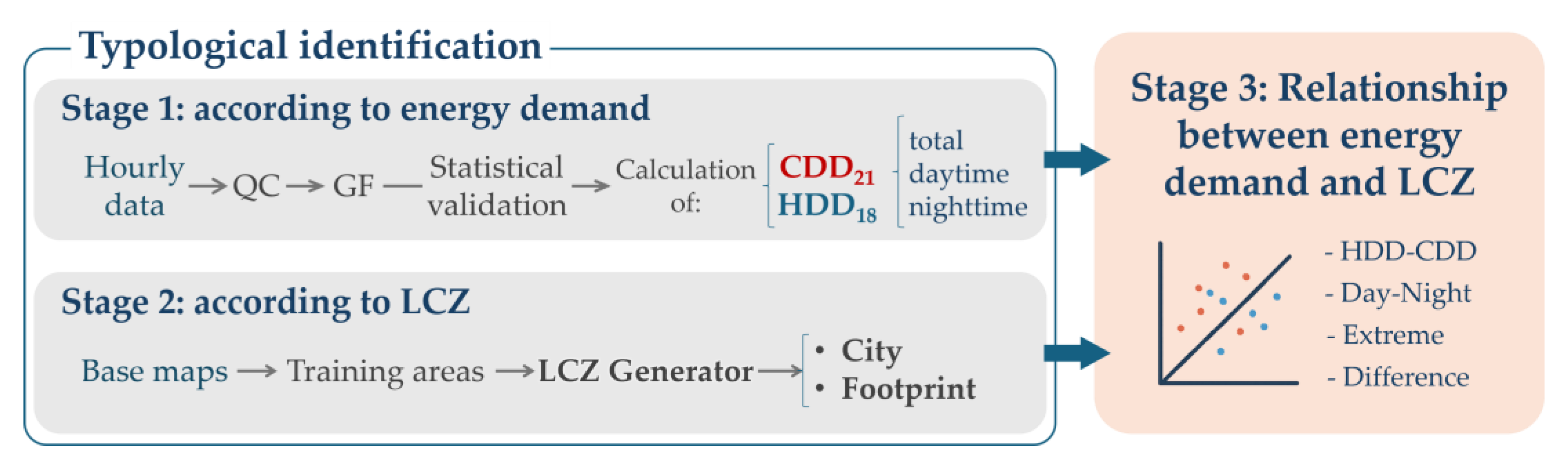
Figure 2.
Box-and-whisker plot of hourly temperature records (°C) for each station during winter and summer.
Figure 2.
Box-and-whisker plot of hourly temperature records (°C) for each station during winter and summer.
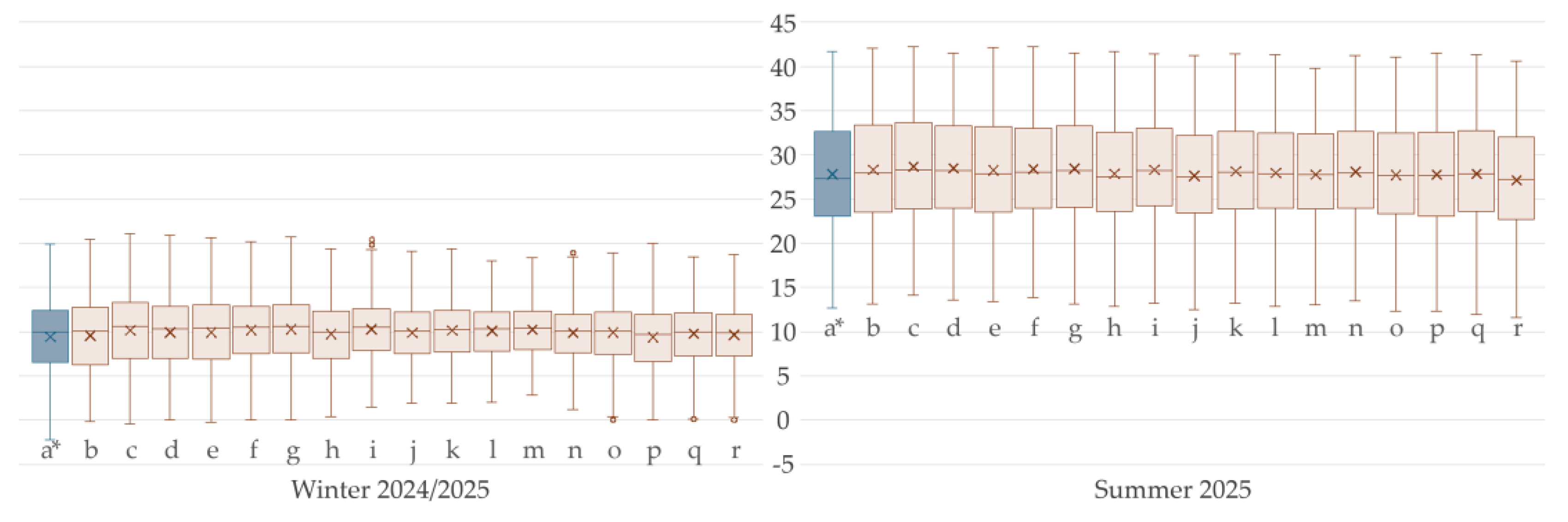
Figure 3.
Pearson correlation coefficient between sensor pairs based on hourly temperature. Upper triangle: winter; lower triangle: summer; diagonal: stations.
Figure 3.
Pearson correlation coefficient between sensor pairs based on hourly temperature. Upper triangle: winter; lower triangle: summer; diagonal: stations.
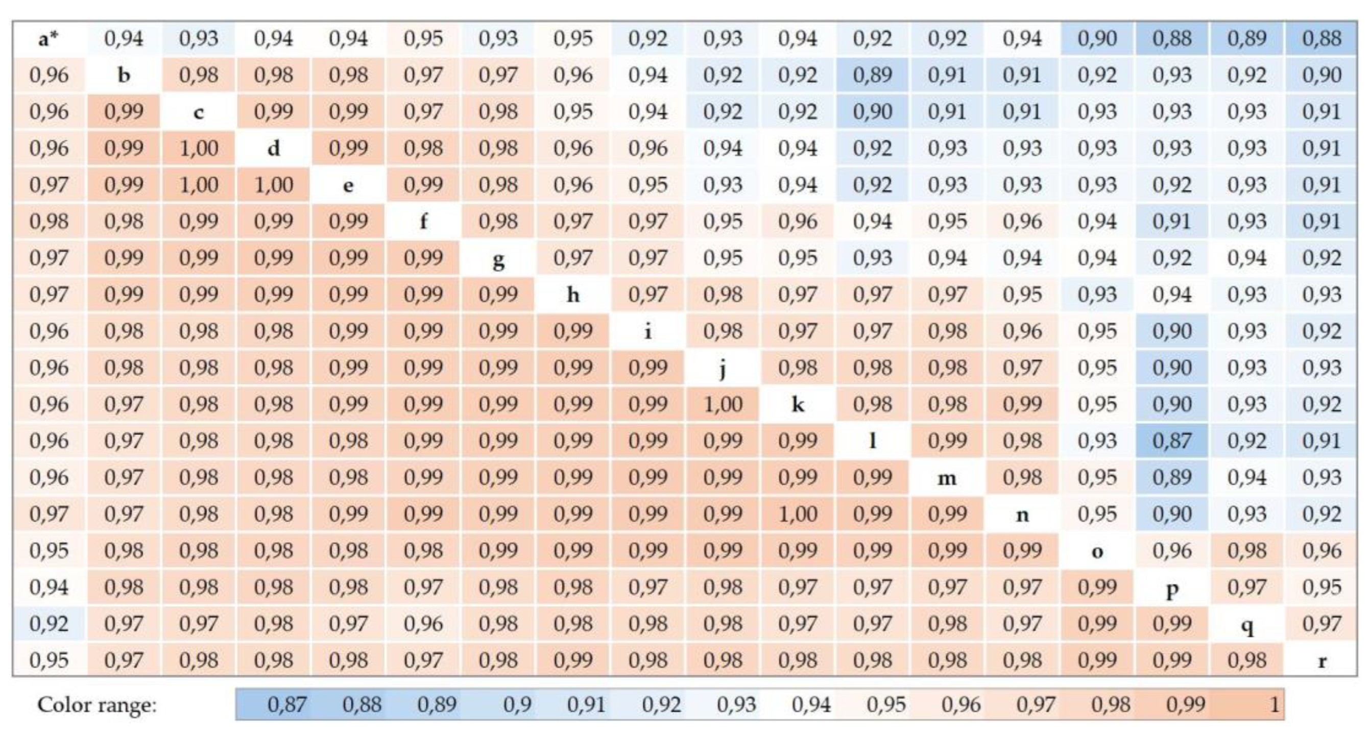
Figure 4.
LCZ identification for the city of Cáceres and location of the hygrothermal stations (“a*” to “r”).
Figure 4.
LCZ identification for the city of Cáceres and location of the hygrothermal stations (“a*” to “r”).
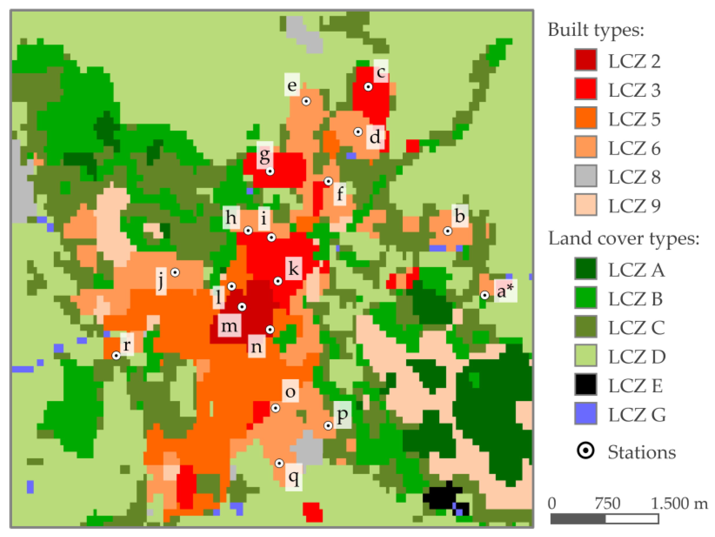
Figure 5.
LCZ distribution within each footprint, showing the proportion of green and built-up areas and the dominant LCZ for each station.
Figure 5.
LCZ distribution within each footprint, showing the proportion of green and built-up areas and the dominant LCZ for each station.
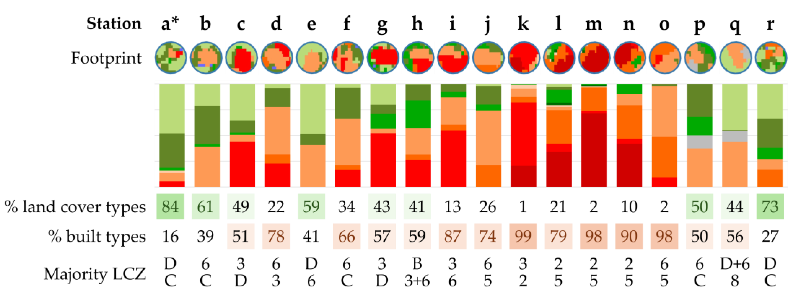
Figure 6.
Relationship between CDD and HDD. The stations are represented through their footprints.
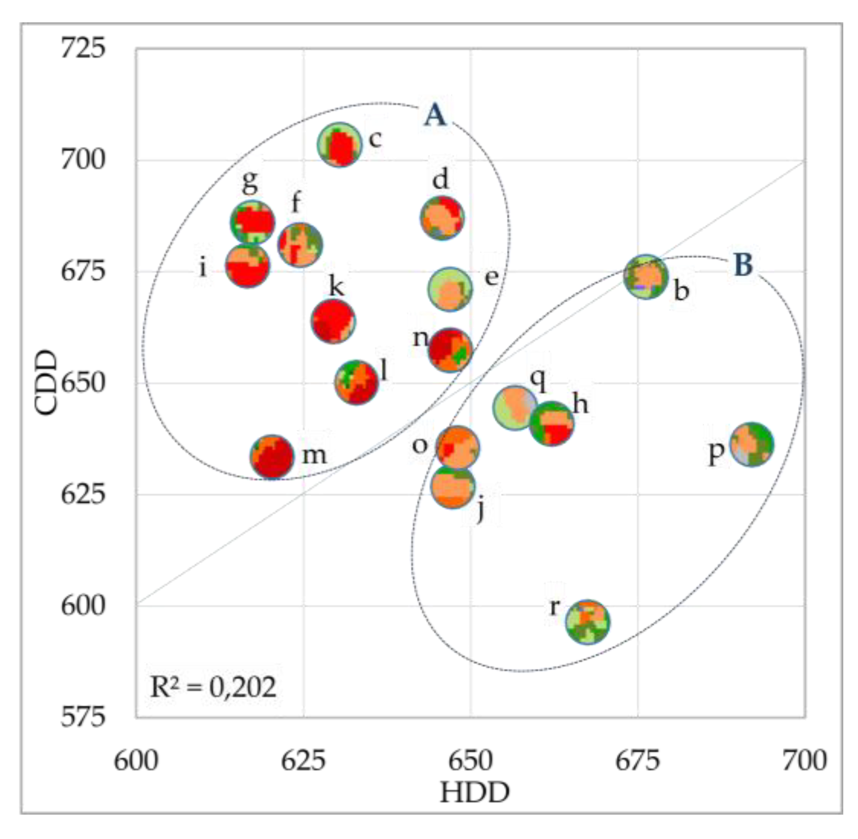
Figure 7.
Relationship between CDD and HDD: (a) daytime; (b) nighttime. The stations are represented through their footprints.
Figure 7.
Relationship between CDD and HDD: (a) daytime; (b) nighttime. The stations are represented through their footprints.
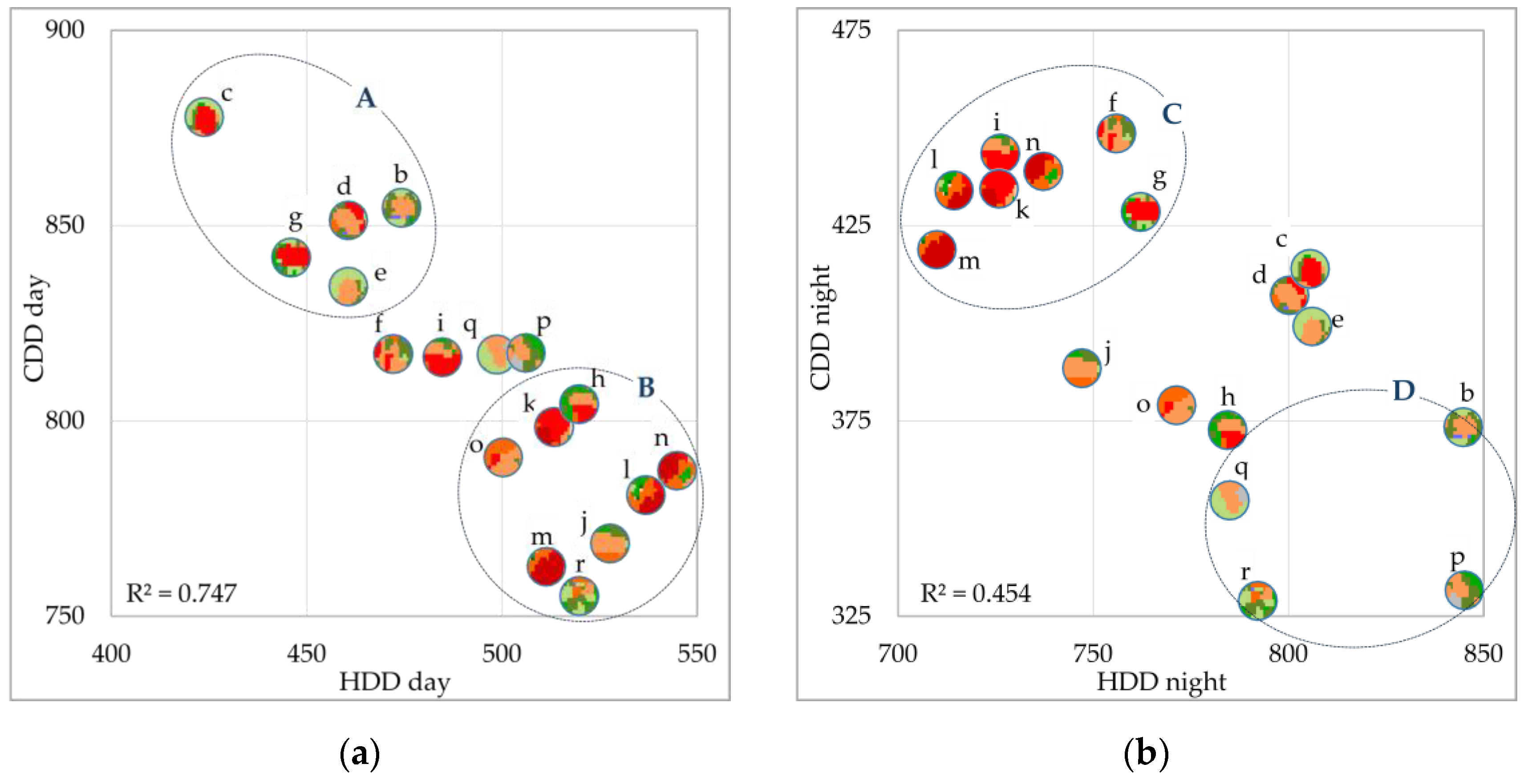
Figure 8.
Relationship between daytime and nighttime values: (a) HDD; (b) CDD. The stations are represented through their footprints.
Figure 8.
Relationship between daytime and nighttime values: (a) HDD; (b) CDD. The stations are represented through their footprints.
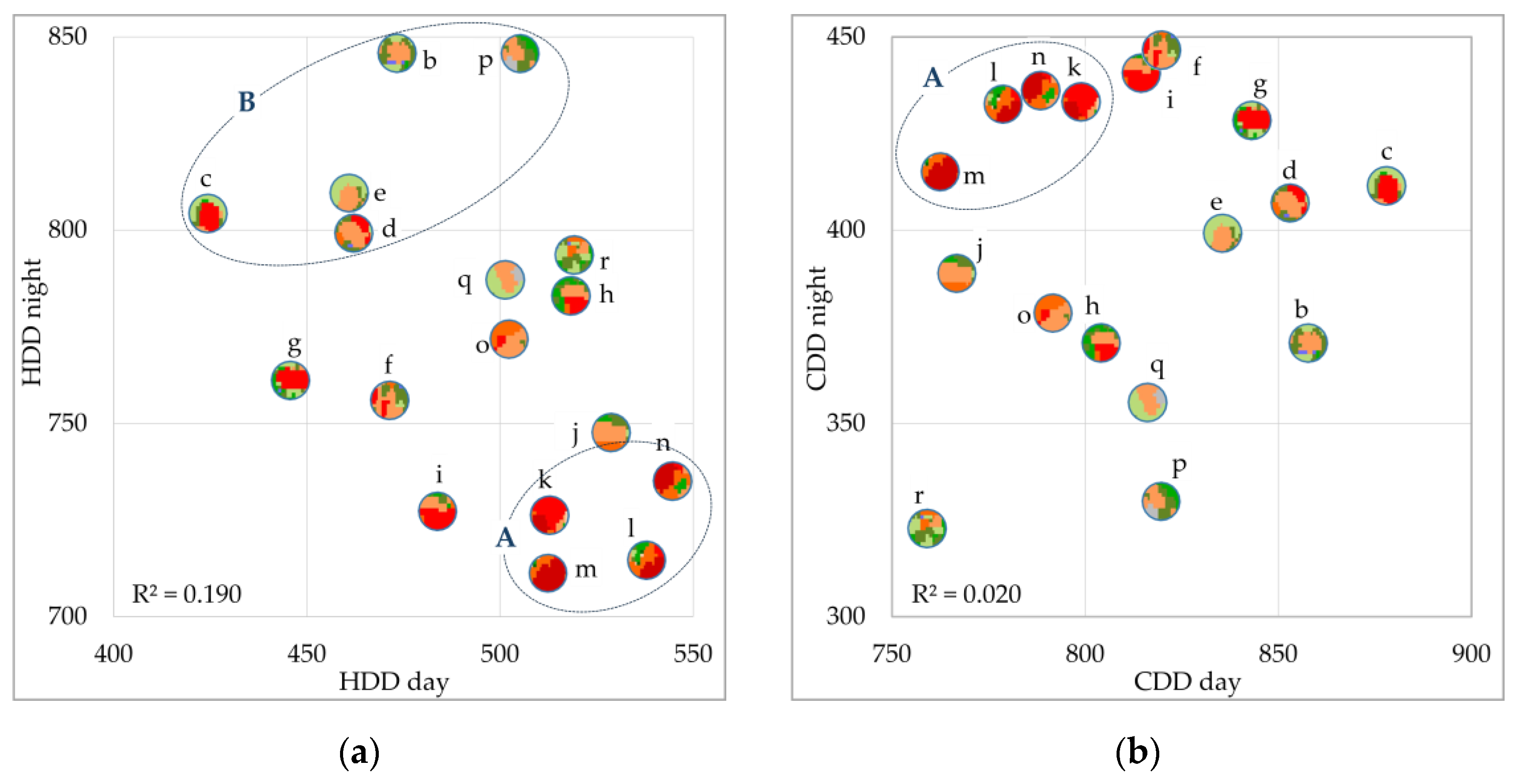
Figure 9.
Relationship between HDD and CDD differences. The stations are represented through their footprints.
Figure 9.
Relationship between HDD and CDD differences. The stations are represented through their footprints.
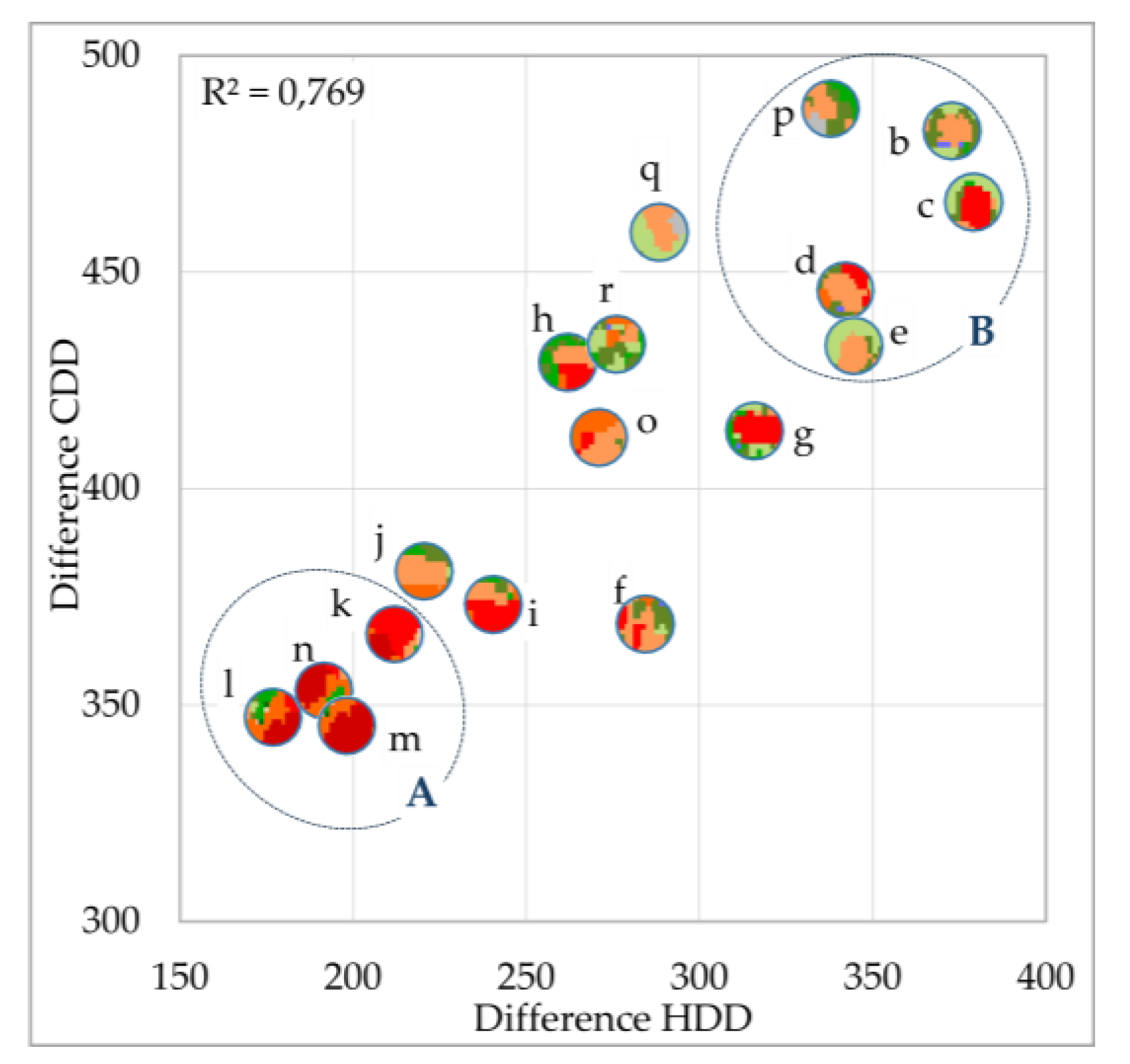

Table 1.
Percentage of records from each hygrothermal station during the studied seasons.
| % | a* | b | c | d | e | f | g | h | i | j | k | l | m | n | o | p | q | r |
| W 1 | 96 | 94 | 95 | 95 | 95 | 95 | 86 | 90 | 95 | 68 | 79 | 88 | 94 | 95 | 93 | 90 | 95 | 79 |
| S 2 | 84 | 100 | 100 | 99 | 100 | 98 | 90 | 100 | 100 | 100 | 90 | 80 | 99 | 100 | 97 | 96 | 96 | 89 |
1 W = winter; 2 S = summer.
Table 2.
HDD and CDD values (°C·day) for each station.
| HDD | CDD | |||||||
| Station | total | day | night | Dif *1 | total | day | night | Dif *1 |
| a* - AEMET | 687 | 546 | 807 | 261 | 634 | 763 | 419 | 344 |
| b | 676 | 474 | 847 | 373 | 675 | 856 | 373 | 483 |
| c | 630 | 424 | 804 | 380 | 704 | 878 | 414 | 464 |
| d | 646 | 461 | 802 | 341 | 687 | 853 | 409 | 444 |
| e | 647 | 460 | 806 | 346 | 672 | 834 | 401 | 433 |
| f | 625 | 471 | 755 | 284 | 681 | 819 | 450 | 369 |
| g | 618 | 446 | 763 | 317 | 687 | 843 | 429 | 414 |
| h | 662 | 519 | 784 | 265 | 642 | 804 | 373 | 431 |
| i | 616 | 485 | 727 | 242 | 677 | 817 | 443 | 374 |
| j | 648 | 529 | 748 | 219 | 626 | 768 | 389 | 379 |
| k | 630 | 514 | 727 | 213 | 663 | 800 | 434 | 366 |
| l | 633 | 537 | 714 | 177 | 650 | 780 | 433 | 347 |
| m | 620 | 512 | 711 | 199 | 633 | 763 | 416 | 347 |
| n | 648 | 544 | 736 | 192 | 657 | 788 | 439 | 349 |
| o | 647 | 501 | 771 | 270 | 635 | 790 | 378 | 412 |
| p | 691 | 506 | 847 | 341 | 636 | 818 | 331 | 487 |
| q | 657 | 501 | 788 | 287 | 645 | 818 | 357 | 461 |
| r | 667 | 520 | 792 | 272 | 595 | 757 | 325 | 432 |
| Mean ± SD | 645 ± 21 | 494 ± 34 | 772 ± 42 | 278 ± 65 | 657 ± 28 | 811 ± 35 | 400 ± 39 | 411 ± 48 |
| Difference*2 | 11% | 22% | 16% | 53% | 15% | 14% | 28% | 29% |
*1 Difference between the daytime and nighttime values of the station. *2 Percentage of the difference between the maximum and minimum values of the local network station set with respect to the maximum value.
Disclaimer/Publisher’s Note: The statements, opinions and data contained in all publications are solely those of the individual author(s) and contributor(s) and not of MDPI and/or the editor(s). MDPI and/or the editor(s) disclaim responsibility for any injury to people or property resulting from any ideas, methods, instructions or products referred to in the content. |
© 2025 by the authors. Licensee MDPI, Basel, Switzerland. This article is an open access article distributed under the terms and conditions of the Creative Commons Attribution (CC BY) license (http://creativecommons.org/licenses/by/4.0/).
Copyright: This open access article is published under a Creative Commons CC BY 4.0 license, which permit the free download, distribution, and reuse, provided that the author and preprint are cited in any reuse.


