Accelerating Time-Domain Fatigue Screening of Offshore Structures with an Integrated Unit Load Response and Submodelling Workflow

Glib Ivanov; Gwo-An Chang; Ding-Peng Liu; Kai-Tung Ma

doi:10.20944/preprints202512.0202.v1

Submitted:

01 December 2025

Posted:

03 December 2025

You are already at the latest version

Abstract

Time-domain fatigue analysis of floating offshore wind turbines (FOWTs) is accurate but often prohibitive for early-stage design. The Unit Load Response (ULR) method, based on linear superposition, offers an efficient alternative, but its application to large, shell-based structures with complex distributed loads remains a challenge. We propose a workflow that integrates ULRs with force-based submodelling to enable whole-structure fatigue screening at design cost. Two key innovations make it practical: (i) A "Virtual Test Rig" is used to create a computationally fast, stiffness-equivalent simplified global model for extracting boundary loads. (ii) A ULR catalogue is generated for a detailed local submodel, which includes a trilinear interpolation scheme (with water height, pitch, roll) to efficiently handle complex, wave pressure fields. The workflow is first verified on a canonical portal frame and then applied to a full-scale semisubmersible FOWT. Across 14 critical locations, the reconstructed stress time histories match the submodel with a median bias ≈ of approximately −3.8% to −4.9%, and the stress and fatigue rankings are preserved, with Kendall’s τ-a ≥ 0.7 at stress concentrations and τ-a ≥ 0.8 overall. Compared to classic step-by-step submodelling, the method achieves ~13-29 times lower wall-clock effort and produces outputs that are otherwise impractical at scale (e.g., full-hull damage maps), enabling earlier, more informed fatigue-driven design decisions.

Keywords:

fatigue analysis

;

unit load response (ULR)

;

floating offshore wind turbine (FOWT)

;

submodelling

;

time-domain analysis

;

fatigue screening

Subject:

Engineering - Marine Engineering

Introduction

Fatigue analysis has become a practical design concern due to cyclic loading, limiting the service life of welded steel structures, offshore platforms, bridges, and ship hulls. For example, experience from FOWT demonstrators in Japan suggests fatigue is more critical than expected [1], and a 2025 Lloyd’s Register report warns that some fixed-bottom wind farms may not adequately account for fatigue [2,3]. Valid fatigue assessment is often constrained by time or methodological limits. Over the last two decades, methods have ranged from frequency-domain formulations that use spectral density functions to detailed time-domain simulations. A comparative review by Muñiz-Calvente et al. [4] found frequency-domain methods computationally attractive but prone to underpredict damage at complex welded joints or under nonlinear loading. Ringsberg et al. [5] investigated (i) whether a nonlinear analysis would be required; (ii) whether frequency-domain analysis suffices; (iii) how global (whole-ship) and local (stiffener-to-shell) finite element (FE) fatigue results compare. Using a 4,400-TEU container ship model, they showed that the global model could identify the same low-fatigue life areas as the combination of multiple local models, facilitated by the ship’s fatigue map, conceptually similar to the one in Figure 1. For all wave directions (0°–180° in 15° increments), critical fatigue locations were identified at the midship hatch corners, the engine room bulkhead, and the bilge. Plastic strain appeared only in a few tiny regions with negligible impact on fatigue life; they thus concluded that linear time-domain analysis (linear geometry and material) is sufficient for screening.

Fatigue screening of offshore floating systems remains challenging due to distributed, time-varying pressure fields and coupled motion responses. Gao et al. [6] presented a time-domain stress analysis for a wind-turbine floater under combined environmental loads, showing that peak stress responses at certain nodes (e.g., fairlead attachments, tower base) are significantly larger than those predicted by global models using simplified load partitioning. Haselibozchaloee et al. [7] reported that welded details, tubular joints and connections are most prone to fatigue failure, and that existing methods may fail to capture global structural interactions under combined wind-wave loading. Therefore, corrections for combined wind-wave nonlinearities have been incorporated into spectral methods [8] to evaluate fatigue damage for floating support structures. Reliability-based approaches and sensitivity analysis for monopile foundations [9] and mooring-chain fatigue [10] demonstrate that waves and wind turbulence primarily drive damage, and that simplified spectral assumptions can either under- or overestimate fatigue, depending on variations in environmental statistics (e.g., wave steepness, peak period, turbulence intensity). Together, these works demonstrate that fatigue strength is strongly influenced by local geometry, weld penetration, loading sequence, and environmental variability.

A recurring limitation is that fatigue evaluations are generally confined to a small set of predetermined locations, such as weld roots, rib-to-deck joints, mooring attachments, or other “known hotspots” [6,11]. While this is useful, it implies the risk of missing other critical areas. Likewise, most of the FOWT fatigue studies are limited to the mooring system [12,13] since it is one of several historical failure modes, leaving hull and tower weld details comparatively underexplored [14]. To our knowledge, none of the above studies perform fatigue checks at all finite-element mesh nodes by reconstructing local stress histories everywhere, primarily due to prohibitive computational cost [11]. Similar limitations were highlighted in an extensive literature review by Rappe et al. [15], who developed an updated algorithm to map aero-hydro-servo-elastic simulation loads to a FOWT FE model and in [16], where researchers compared frequency and time domain method fatigue damage across 16000 hotspots. To address these gaps, we adopt a load-mapping procedure from AQWA and develop a unit load responses (ULRs)-based screening method that reconstructs node-wise stress histories across the entire structure.

Recent studies have shown that superposing unit load cases can drastically reduce FE runtime while maintaining accuracy in various structures, including an aeroplane wing [25], a mooring bracket [26], and an elastomeric shaft bushing that required advanced interpolation [17]. This enables whole-structure fatigue scanning rather than reliance on pointwise stress concentration monitoring, improving the chance of detecting unexpected damage locations and providing a more comprehensive assessment of fatigue life. Nevertheless, these studies focus on small-scale structures composed of solid elements with simple applied forces/moments and report near-zero errors (also consistent with our prior results [18]). Direct application to large offshore structures modelled with thin shell elements and subjected to distributed field loads (e.g., water pressure) remains nontrivial for pressure-field representation. Therefore, in this study, we develop a ULR-based fatigue-screening workflow for floating offshore structures that (i) reconstructs node-wise stress histories under combined wave, mooring, and turbine loads, and (ii) enables whole-structure fatigue checks at design-stage cost. The method precomputes ULRs for representative boundary and pressure conditions and then reconstructs stresses by linear superposition [19] with low-dimensional pressure interpolation. We evaluate accuracy against a detailed submodel, compare stress and fatigue errors, and examine the robustness of their ranking. The remainder of the paper is structured as follows: Section 2 reviews the fatigue screening methods and introduces the proposed method. Section 3 verifies the proposed method and load mapping using simple models. Section 4 presents a case study of FOWT fatigue analysis, showing the results of stress, accumulated fatigue damage and ranking. Section 5 discusses applicability, limits, and sensitivity to time resolution and pressure-grid design.

Methodology

Submodelling Method

In this study, we compute ULRs using a force-based submodel. Submodeling, introduced by Sun et al. [20], has been applied to the structural design of ships and offshore platforms [21,22]. More recently, Starr et al. [23] compared structural analysis methods for floating-wind tension-leg platforms and found that submodeling achieved close agreement with high-fidelity analyses, supporting its use as a reference method here.

Consider the surface body in Figure 2 subjected to boundary shear and an out-of-plane Z-direction load (global model). A global analysis alone yields stresses that are too coarse for fatigue assessment [22]. Let EFGH denote the region of interest. We cut out a local domain bounded by rectangle ABCD and remesh it finely (local model). By Saint-Venant’s principle, the stress field in EFGH is insensitive to details far from the applied loads if equivalent resultants are imposed on the cut boundary. Accordingly, we apply the cut-boundary forces and moments extracted from the global model along ABCD; any remaining external Z-load is applied directly to the local domain. The local domain is chosen larger than EFGH so that boundary effects are confined near ABCD and do not contaminate stresses in the region of interest.

Regarding submodelling, two boundary-mapping approaches are common: displacement-based and force-based. Narvydas et al. [24] showed that displacement-based submodels tolerate very coarse global meshes but can produce inconsistent results when local stiffness differs between the global and local models. Because our simplified global model intentionally alters local stiffness, we adopt a force-based submodel, which in turn requires a mesh-convergence study of the cut-boundary forces/moments extracted from the global analysis. In addition, the cut-boundary distance from the region of interest is a critical parameter for accuracy. For the submodel used in this study, the optimal boundary placement, the global-force and local-mesh convergence checks, and other validity assessments were already established in our previous work [25] and are followed in this study.

Unit Load Response Method

Figure 3 summarizes the three stages used to obtain node-wise stress histories: (i) global-model load extraction, (ii) submodel ULR generation, and (iii) stress-history reconstruction. The reconstructed histories are then used for fatigue calculations or design strength checks. To apply the ULR approach to shell-dominated offshore structures with distributed loads, we employ three techniques: (i) ULR combined with submodelling, so ULRs are computed only on the detailed local model; (ii) global-model simplification via a Virtual Test Rig, to obtain reliable interface loads at low cost; and (iii) pressure-field interpolation, for which we compare candidate algorithms and select settings suitable for offshore applications. These choices enable rapid stress-history reconstruction but introduce approximation errors. We therefore quantify accuracy alongside speed; an error-free result is not expected—nor required for screening—as shown in related studies [19,26,27].

The proposed ULR method is summarised as follows:

(i): On the local (submodel) mesh, compute unit load responses for each load case $k$ (forces = $1 N$ ; moments = $1 N m$ ) and direction. Let $σ_{i}^{(k)} (n)$ denote the resulting component stress at node $n$ for stress component $i \in \{1, \dots, 6\}$ (e.g., $σ_{x x}, σ_{y y}, σ_{z z}, τ_{x y}, τ_{y z}, τ_{z x}$ ).
(ii): For a given time history of loads $L_{k} (t)$ (cut-boundary resultants from stage (i) of the workflow), reconstruct the nodal component stresses by linear superposition:

σ_{i} (n, t) = \sum_{k} L_{k} (t) \times σ_{i}^{(k)} (n)

(1)

where ULRs are time-independent and computed once; only the scalar weights

L_{k} (t)

vary with time.

(iii): From the components ${σ_{i} (n, t)}$ , compute any required derived measure at node $n$ —e.g., von Mises, principal, or absolute maximum principal stress—for each time step to obtain the stress history. In the full floater study, Equation (1) is evaluated at every mesh node. Because Equation (1) separates precomputed spatial responses $σ_{i}^{(k)} (n)$ from time-varying scalars $L_{k} (t)$ , the method scales efficiently to long simulations and is well suited to time-domain fatigue calculations.

Consider the top beam

B C

of a portal frame with fixed-base columns (Figure 4). The beam of span

L = 3 m

carries a uniform load

q = 20,000 N / m

. Section properties are

I_{x x} = 2.16 \times 10^{- 4} m^{4}

and

A = 1.84 \times 10^{- 2} m^{2}

. Stresses are evaluated at midspan on the tension fibre,

y = 0.15 m

from the neutral axis. The frame is third-degree statically indeterminate; the force method gives the bending-moment diagram in Figure 17 (right). For normal stress

σ_{x x}

, only axial force

N

and bending moment

M

at the section contribute. The ULRs at a node

n

are

{U L R}_{M} (n) = \frac{y}{I_{x x}} [\frac{P a}{N m}], {U L R}_{N} (n) = \frac{1}{A} [\frac{P a}{N}]

(2)

ULRs are purely geometric and time-independent. With generalized loads

M

and

N

from the global solution, the nodal stress follows by linear superposition:

σ_{x x} (n) = M {U L R}_{M} (n) + N {U L R}_{N} (n) .

(3)

For the portal under UDL, the midspan values are

M_{mid} = (5 q L^{2}) / 72

and

N_{mid} = q L / 12

. Substituting

q, L, y, I_{x x}, A

gives

σ_{b e n d i n g} = \frac{M y}{I_{x x}} = \frac{(\frac{5 q L^{2}}{72}) \times 0.15}{0.000216} = 8.681 M P a σ_{a x i a l} = \frac{q L}{12 A} = \frac{60000}{12 \times 0.0184} = 0.270 M P a σ_{x x, m a x} = σ_{b e n d i n g} + σ_{a x i a l} = 8.951 M P a

(4)

Interpolation of Wave and Static Pressure

Hydrostatic and hydrodynamic pressures are distributed loads: the value at each surface node depends on the instantaneous free-surface elevation and attitude of the body. A conventional ULR strategy (one ULR per node and per load case) would therefore require hundreds of thousands of ULRs. We address this by replacing per-node ULRs with a parametric pressure basis and reconstructing stresses by interpolation in a low-dimensional space. Static pressure is defined by water depth, while time-varying wave pressure is described by a small set of body motion parameters. In this study, we use heave, pitch, and roll as the interpolation axes. We precompute ULRs at selected combinations of these parameters (a sparse grid). Each grid point represents a full pressure field applied to the local model, and its nodal stress response is stored.

For each time step, the current heave, pitch, and roll are located within the grid cell that encloses them. The nodal stresses are then obtained by trilinear interpolation of the precomputed ULRs at the eight surrounding grid points (Figure 5). This yields node-wise stress histories without generating a separate ULR for every surface node. We use a mixed (non-uniform) grid, adding points only where sensitivity is highest (e.g., along edges with steep pressure gradients), following the trilinear scheme of Canelhas et al. [28]. The operating envelope is defined based on the global simulation; points outside this envelope are flagged for grid extension rather than being extrapolated. This keeps the catalogue compact, controls interpolation error, and preserves the speed advantages of the ULR workflow.

Three interpolation strategies are evaluated against the reference 3D frame submodel solution in this study:

HPR-M (mixed grid). A non-uniform grid in Heave–Pitch–Roll (HPR) space with local refinement near the most probable attitudes (small pitch/roll). This catalogue contains 1366 ULRs. Coarse cells cover the full operating envelope; fine cells densify the low-load region where the floater spends most of its time.
HPR-C (coarse grid). A uniform HPR grid covering the same envelope without local refinement, totalling 525 ULRs.
H (heave-only). A one-parameter interpolation that varies the effective water level while neglecting pitch and roll. This uses 21 ULRs spanning from −10 to +10 m relative to still water. The simplification is motivated by the small-angle regime (pitch/roll typically ≤ ~2°).

Figure 6 illustrates the construction of the approximated pressure fields by manipulating the free surface across the chosen grid points. For each time step, we (i) extract the pressure-state parameters (heave, pitch, roll and effective water level) from the global simulation; (ii) locate the enclosing H–P–R grid cell and compute trilinear (or unilinear) interpolation weights (e.g., [height0;pitch0;roll3], [h0;p1;r3], [h0;p0;r6], [h0;p1;r6], [h1;p0;r3], [h1;p1;r3], [h1;p0;r6], [h1;p1;r6].); and (iii) read the precomputed pressure ULRs at the cell’s corner points and interpolate nodal stress components, which are then summed with other load contributions. The pressure amplitude is represented entirely by the interpolation weights, so no additional scaling is applied at this stage.

Fatigue Analysis

Node-wise stress histories are obtained either from the reference submodel or from the ULR-based reconstruction described earlier. The same time window and sampling settings are used in both methods to ensure a like-for-like comparison. In a sensitivity analysis of ship fatigue problem [29], it is found that loads mapped from a 20-minute time-domain hydrodynamic analysis yielded nearly the same fatigue damage as a 3-hour run. For the time step, 0.5 s is recommended to balance accuracy and cost. Given the similarity in wave-load characteristics, this finding might be applicable to FOWT and other structures. Therefore, each fatigue bin was simulated for 20 min with time step of 0.5 s in this study. Boundary forces/moments for the submodel were recorded at the same cadence to preserve phase. The local submodel employed inertia relief, as demonstrated by our previous work [25]. Fatigue was evaluated from node-wise stress histories using rainflow counting [30,31] and Palmgren–Miner [32] accumulation with DNV-RP-C203 [33], curve W3 (seawater with cathodic protection); standard thickness/mean-stress options were applied where relevant.

For the case study, a single fatigue bin was used, with a wind speed of 20.33 m/s, a 1.5 m wave height, a 5.5 m wave period, and a wave-wind misalignment of 45 degrees.

Method Verification—3D Frame

Unit Load Response

The (global) portal frame was re-analysed in Ansys Mechanical and benchmarked against the closed-form beam solution. The bending-moment distribution (Figure 4) from FEM matches the analytical diagram, and Table 1 summarises stress/moment agreement for beam- and shell-element models. To enforce a rigid-joint assumption in the shell representation, we introduced internal stiffeners at the beam–column connection. The stiffened shell model reproduces the analytical mid-span bending moment within 0.51%, confirming structural equivalence. The axial force in the beam model is 4810 N versus 5000 N analytically; the shear force is 100 N versus 0, reflecting formulation differences rather than modelling error. We then assembled a 3D frame from four identical 2D frames (Figure 7), using 1 mm internal joining brackets in the shell model. For Beam 1, the 3D shell solution is the closest to the analytical result (Table 1). Beam 2 uses the same section but a slightly different connection; because the hollow rectangular section is not symmetric with respect to both section axes, its response differs and lies outside the force-method assumptions. Accordingly, Beam 2 is validated by comparing shell and beam FEA only, which show close agreement. Finally, the 3D shell model reveals non-uniform stress over a given section/elevation (e.g., along the top plate), a shear-lag effect naturally captured by finite elements but not represented in the baseline analytical solution (and not required for the present checks).

With the global 3D beam and shell frames validated against the analytical solution, we proceed to submodelling and ULR modelling under a composite load case that captures (i) forces entering and leaving the local domain, (ii) both distributed and point loads, and (iii) axial, shear, bending, and torsional loads (Figure 7, right). Verification is based on equivalent von Mises stresses at 12 preselected hot spots—corner stress concentrations at the beam–column joint (Top), mid-height of the column (Mid), and the fixed support (Bot) as shown in Figure 7—reflecting strength and fatigue-critical locations. The global shell model is taken as the reference for error evaluation, as it best represents the physical structure. For submodelling, we employ fixed support submodels with three load-application schemes: (i) reactions extracted from the global beam model; (ii) reactions extracted from the global shell model; and (iii) as in (ii) but using rigid remote-point cut boundaries. Table 2 summarizes the resulting stress errors across all points. Comparing results obtained using loads extracted from beam and shell global models, the shell load submodel shows consistently good results in all top, middle, and bottom sections, while the beam load model only shows good results in the middle (far from the connection and support). This difference in extracted loads from the shell and beam global models is seen in Table 3; while the main forces are the same, there can be a significant difference in the small-magnitude MX and MZ moments due to the formulations of beam and shell elements. This difference is amplified when multiplied by the ULR.

To understand the sources of the Table 2 errors, we decompose them into three contributors—(i) ULR boundary-condition error, (ii) submodelling boundary-proximity error, and (iii) distributed-load error—and examine them in isolation, beginning with the ULR boundary condition. In the global model, the frame is fixed at the base of C1; however, this support is outside the local domains used to compute ULRs, so an auxiliary boundary condition is required. Figure 8 defines three candidate boundary conditions, and for each boundary, the cut section is modelled either as deformable or as artificially rigid via a multi-point constraint (remote point in ANSYS), yielding six boundary-condition combinations. All models are evaluated under four load cases: (i) top-surface distributed load only, (ii) the combined loading as shown in Figure 7, (iii) the point moment only as shown in Figure 7, and (iv) the combined case (ii) with the distributed load removed. For every node, equivalent von Mises stresses from the local models are compared to the global shell reference, and the signed percentage errors are plotted in Figure 9.

For screening, the correct ordering of hot spots often matters more than exact stresses. To evaluate whether the proposed approach could incorrectly rank nodes, we used Kendall’s τ-a, an established rank-correlation metric [34], alongside stress errors.

Nodes near the boundaries were excluded from τ-a to remove boundary effects. From the results in Table 4, inertia-relief boundary conditions perform better than the other conditions, yielding a 1.86% median absolute error across the four load cases. With inertia relief enabled, the choice of cut-boundary location and whether the section was modelled deformably or via a remote-point constraint had negligible influence. In contrast, a fixed-bottom condition required a substantially larger submodel and higher cost; accordingly, we select simple inertia relief for the case study. Load-case sensitivity further shows that, when distributed forces are absent, stress errors are ≈0% and node rankings are preserved (τ-a≈1); as the proportion of distributed loading increases (combined < distributed), stress errors rise and ranking fidelity degrades, identifying distributed loads as the principal challenge for ULR, addressed next.

The large gap between the median and mean errors in Table 4 may arise from boundary-condition artefacts—unphysical stress spikes localised near the cut, as shown in Figure 9—so model cuts should be placed well away from the region of interest (the beam joint). Figure 8 quantifies boundary-proximity effects by tracking von Mises stresses at hot-spot nodes (region of interest) and at four bottom-corner control nodes (expected to be insensitive) under seven unit-load cases: six global end loads (three 1 N forces and three 1 Nm moments applied at the far end of B4) and a 1 Pa uniform pressure on the top surface (the same basis used for ULR extraction). Cut loads are sampled at multiple distances and applied to a fixed-bottom local model (with pressure also applied locally). Results show near-zero stress errors for all non-pressure unit loads—even at the minimum boundary distance—with errors increasing as the cut moves closer, while the bottom control nodes remain unaffected. In contrast, the distributed-pressure case exhibits non-zero, irregular errors even for distant cuts, motivating the alternative treatment of pressure ULRs development.

Figure 10. Stress results for global and smallest local model when loaded by distributed pressure load. Green lines indicate cuts where loads are exported to local models.

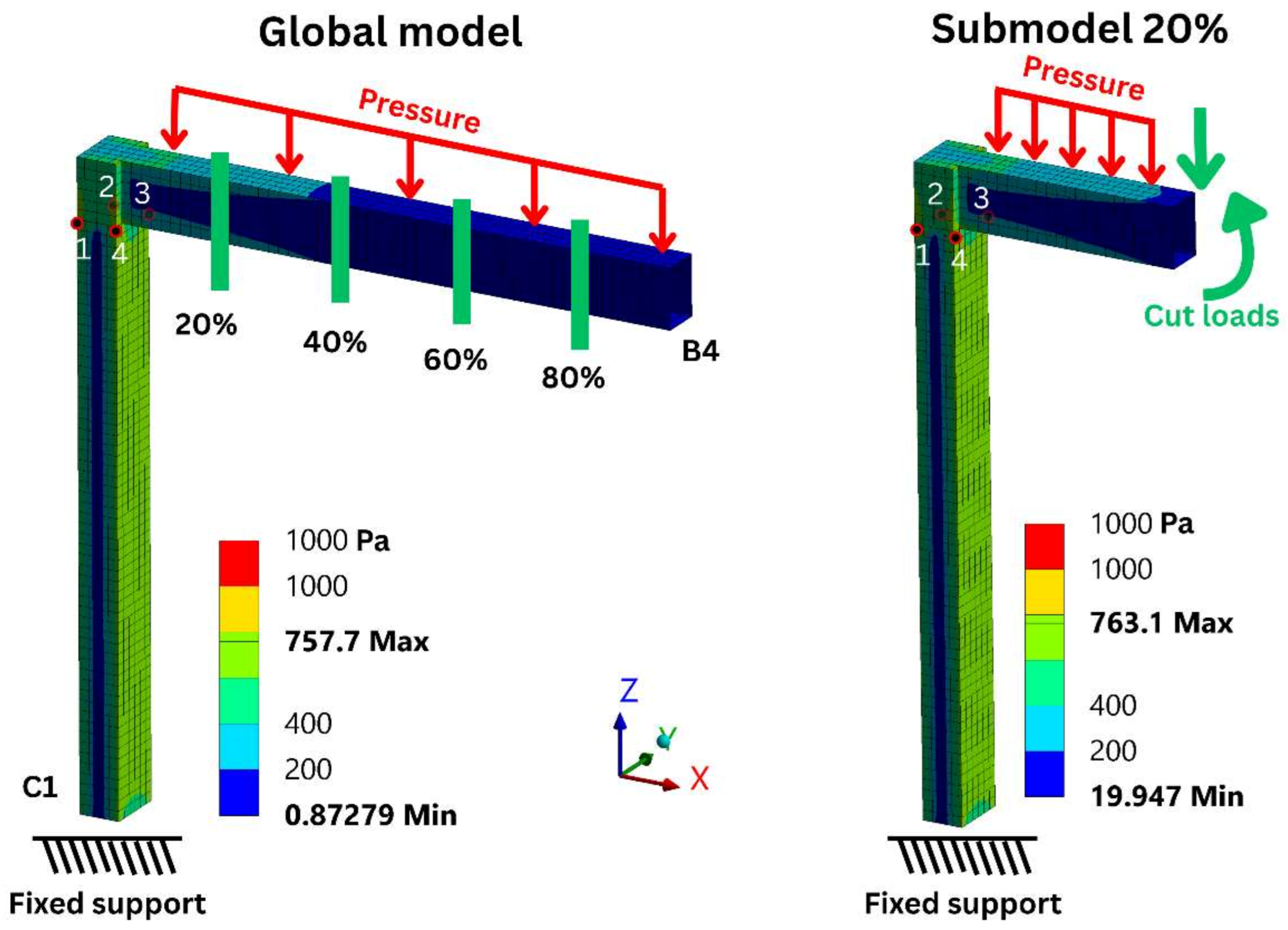
Table 5. Error in stress vs cut boundary distance from 7 unit loads.

	AVERAGE ERROR ACROSS 4 TOP POINTS							AVERAGE ERROR ACROSS 4 BOTTOM POINTS
DISTANCE	FX	FY	FZ	MX	MY	MZ	P	FX	FY	FZ	MX	MY	MZ	P
100%	0.00%	0.00%	0.00%	0.00%	0.00%	0.00%	0.00%	0.00%	0.00%	0.00%	0.00%	0.00%	0.00%	0.00%
80%	0.00%	0.00%	0.00%	-0.03%	0.00%	0.00%	1.45%	0.00%	0.00%	0.00%	0.00%	0.00%	0.00%	1.43%
60%	0.00%	0.00%	0.00%	-0.01%	0.00%	0.00%	1.08%	0.00%	0.00%	0.00%	0.00%	0.00%	0.00%	1.07%
40%	0.00%	0.02%	0.00%	0.23%	0.00%	0.02%	0.71%	0.00%	0.00%	0.00%	0.00%	0.00%	0.00%	0.71%
20%	0.00%	0.39%	0.00%	0.81%	0.00%	0.40%	0.34%	0.00%	0.00%	0.00%	0.00%	0.00%	0.00%	0.36%

Wave and Static Pressure Interpolation

To isolate interpolation effects, we consider wave pressure only and keep the local-model boundary conditions identical to the reference submodel. We apply the HPR procedure to the 3D frame by parameterizing the free-surface state with three variables—heave, pitch, and roll. The frame stands half-submerged (1.5 m); zero heave corresponds to the nominal waterline at 1.5 m, and heave is between -1.5 m and 1.5 m. Pitch and roll vary within −6° and 6°. A tensor grid of ULRs is precomputed over this domain using 0.5 m and 3° spacing for heave and pitch/roll, respectively, producing 175 wave-pressure ULRs (versus 22 in the original non-pressure study).

Table 6. ULR interpolated stress result error for the 3D frame loaded by hydrostatic pressure.

NODE 1	A H1P6R6	0%	NODE 3	A H1P6R6	0%
	B h-0.25p5r2	2%		B h-0.25p5r2	2%
	C h4p8r0	3003%		C h4p8r0	867%
	D h0.75p-4.5r1.5	-2%		D h0.75p-4.5r1.5	-1%
NODE 2	A h1p6r6	0%	NODE 4	A h1p6r6	0%
	B h-0.25p5r2	-1%		B h-0.25p5r2	-1%
	C h4p8r0	2184%		C h4p8r0	958%
	D h0.75p-4.5r1.5	-2%		D h0.75p-4.5r1.5	-2%

The parameter values and corresponding pressure distributions for the four selected cases are shown in Figure 11. During analysis, if the queried state matches a tabulated point exactly, the corresponding ULR is used directly (Case A); otherwise, states within the grid are obtained by tri-linear interpolation from the nearest tabulated ULRs (Case B and D), and states outside the grid are evaluated by linear extrapolation along the nearest coordinate directions (Case C). Table 10 compares these ULR-based stresses against solutions with the exact applied pressure. Case A yields 0% error, confirming the correctness of the ULR setup. Interpolation is accurate: a typical interior query (Case B) incurs near 1% error, while a deliberately worst-positioned mid-cell query (Case D) reaches 2%—the expected upper bound given the chosen grid spacing. By contrast, extrapolation performs poorly: a far out-of-grid query (Case C) exhibits an error on the order of 10³%. Hence, for hydrostatic pressure loads, the parameter grid must cover the full operating envelope to avoid extrapolation.

It is worth noting that interpolation is only one strategy for handling distributed loads. An alternative—commonly used in the oil and gas sector but largely undocumented in the scientific literature—is a global beam pressure–distribution approach: (1) construct an equivalent global beam model from the global shell model with matched cross-sectional stiffness; (2) map the time-varying wave pressure from AQWA (computed on the global shell) to this equivalent model at each time step; and (3) convert the shell pressures into line loads along the pontoons’ longitudinal axes and along the submerged portions of the columns (top, sides, and/or bottom) at each time step, and treat these line loads as additional ULRs. Having separately quantified interpolation, cut-boundary proximity, and boundary-condition errors, the overall expected stress error can be estimated via standard root-sum-of-squares propagation [35] under an approximate independence assumption. Using median deviations of 2.0%, 1.86%, and 1.45%, respectively, the approximate expected combined error is 3.09%. In the next section, geometry error will also be introduced due to global model simplification.

E [ϵ_{t o t a l}] = \sqrt{ϵ_{i n t e r p o l a t i o n}^{2} + ϵ_{d i s t a n c e}^{2} + ϵ_{b o u n d a r y}^{2} + ϵ_{g e o m e t r y}^{2}}

(5)

Case Study

Selected Offshore Structure

To demonstrate the proposed method, we conduct a case study on the TaidaFloat platform. The applied loads reflect the operational state of the floater and comprise wave-induced dynamic and hydrostatic pressures, ballast pressure, wind-turbine forces and moments, and mooring-line tensions exported from OrcaFlex; application details are summarized in Figure 16. Geometric, structural, and hydrodynamic particulars—including Response Amplitude Operators (RAOs) and the OrcaFlex model setup—are documented in [36,37], and boundary-condition options for this system are discussed in [18]. In this case study, the global model uses perfectly balanced loads with only a cylindrical constraint at the fairlead for numerical stability, whereas the local model employs inertia relief—an effective choice for FOWTs as shown by Rappé et al. [15] and corroborated by our earlier results (Table 4).

Figure 12. Loads applied to the floater finite element model.

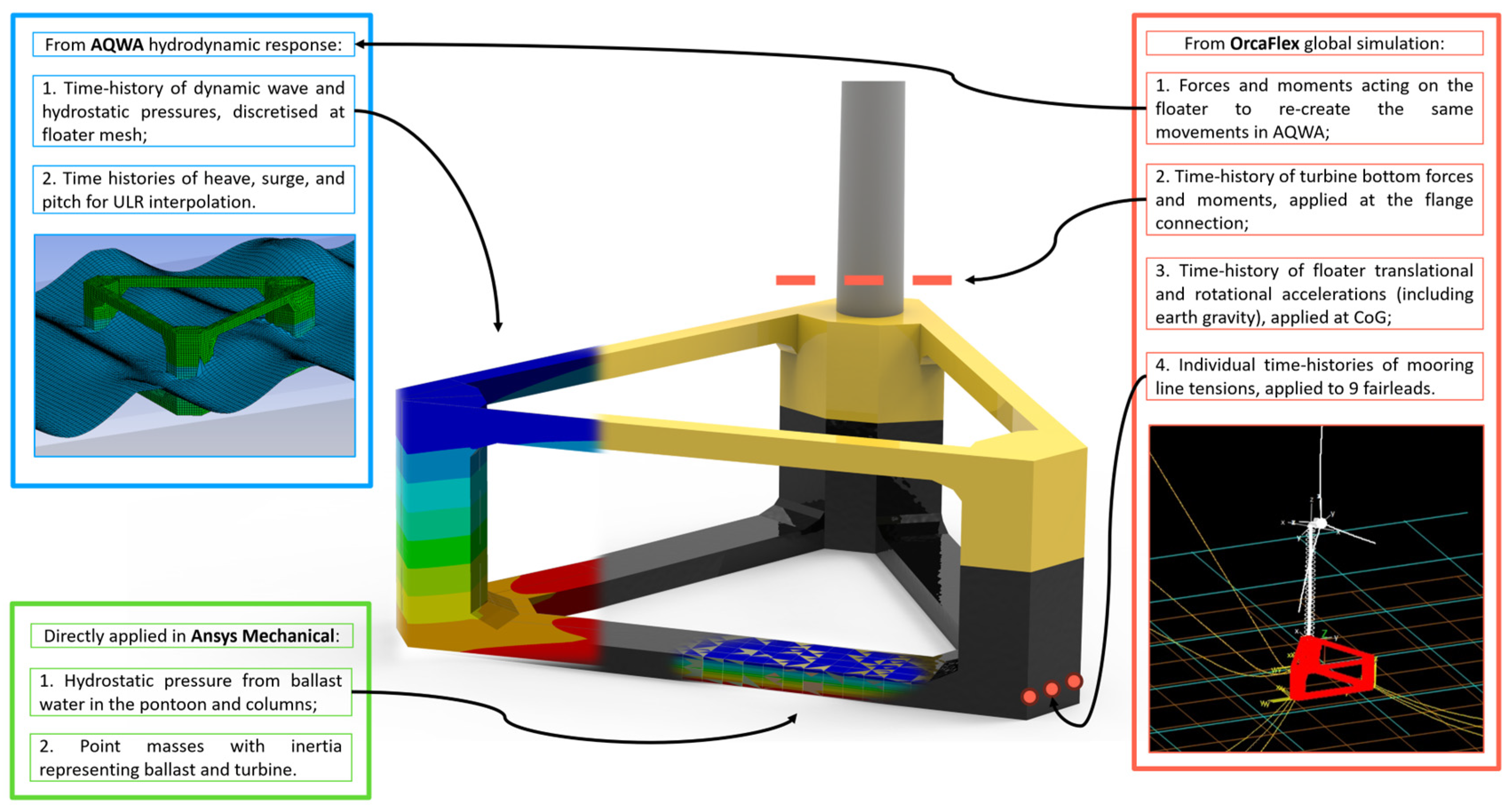
The load histories from OrcaFlex/AQWA are nonlinear, comprising mooring-line tensions, turbine base forces/moments, and hull pressures. Nonlinearity arises from second-order wave kinematics, full-field turbulent wind, current and air drag, line slacking, and a flexible, nonlinear-FE tower. These nonlinearities are captured in the load generation; by contrast, the ULR procedure employs linear FE superposition for the structural response and does not model material or geometric nonlinearities. To improve fidelity over earlier work [5] (which used a ~3 m global mesh due to computing limits), the present global model adopts a 0.23 m element size—about an order of magnitude finer than the simplified model used previously—adequate for strength checks and fatigue screening, albeit coarser than the 0.02 m recommended for hotspot fatigue assessment. This mesh is also substantially finer than the 0.65 m found sufficient in the prior mesh-convergence study [25].

Global Model Simplification

In the verification studies, the local and global models shared identical geometry and mesh. For the full offshore system, however, a simplified global model is required to extract cut-boundary loads. Direct hand-calculation of section properties proved impractical given the complex internal layout—particularly the main column’s bulkheads with varying thicknesses. We therefore adopted a “virtual test rig” (model-calibration) procedure: a coarse-mesh, simplified model is tuned to reproduce the stiffness response of the fine-mesh, detailed model, ensuring structural equivalence. This follows established “equivalent stiffness” practices in complex structural analysis for automotive [38,39] and ocean engineering [40,41].

The floater was partitioned into 33 detachable parts, of which only 10 are unique by symmetry (Figure 17). For each unique part, we prepared (i) a detailed model reproducing the full structural arrangement of the global detailed model (excluding bulkheads located at inter-part joints) with a 0.25 m mesh, and (ii) a simplified model in which all non-web stiffeners were removed, and a 2.5 m mesh was used. Both models were characterised on a virtual test rig: the part was clamped at one end and subjected to prescribed 0.1 m translations at the free end in the global X, Y, and Z directions, mirroring a reduced-scale laboratory cantilever test. This calibration amounts to stiffener lumping, a common practice in ship-structure FEA [41], as illustrated in Figure 18. Initially, reaction forces differed markedly because the changes in geometry altered stiffness. A direct optimisation iteratively adjusted the thicknesses of the simplified parts and reran the virtual test rig until the fixed-end reactions and moments matched those of the detailed model. Depending on the structural details, this required 1–700 simulations, and the coarse 2.5 m mesh kept the iterations fast.

Figure 13. Unique floater parts (left) and example boundary condition application to a part’s local model (right).

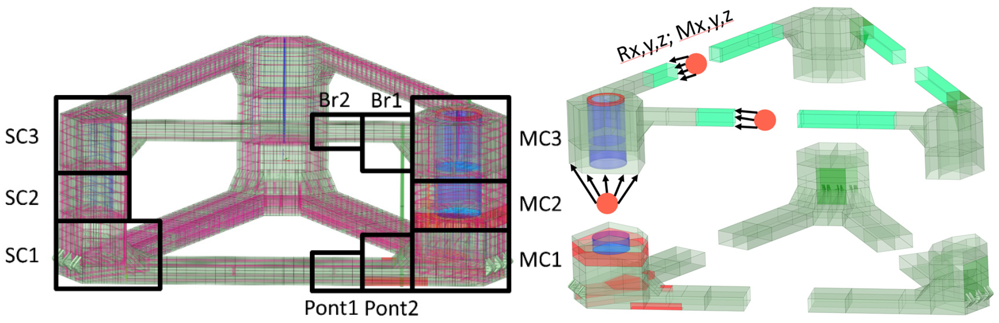
Figure 14. The lumped stiffener simplification principle and its effect on maximum possible mesh size.

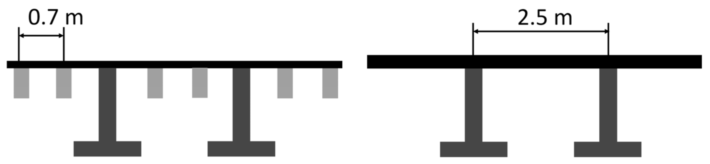
Figure 15 compares directional displacements of the detailed and calibrated simplified models and shows satisfactory agreement. Some parts (e.g., bracing) were straightforward to match in reaction forces, whereas Main Column 2 (MC2) was challenging due to complex internals. Table 7 reports reactions and moments for both models; because exact matching of all six components was unattainable, the goal-seeking optimisation used weighted targets that prioritised the principal loads—longitudinal force (FZ) and longitudinal moment (MY)—identified from the full-scale analysis as two orders of magnitude larger than the other load components. The resulting load-extraction model, assembled from the calibrated parts, minimises geometric part count and uses a coarse 2.5 m mesh, enabling rapid evaluation of global floater loads across all fatigue operational and environmental conditions. These global loads then drive the local-model stress histories and the control submodel.

Ideally, the floater can be divided into 6 parts, as seen in Figure 17(right), which would allow for more mesh refinement. However, to avoid stress distortion at the interfaces between stacked local models, we combined the planned top–bottom column segments into single continuous locals. The floater was partitioned into three local models—Main Column, Side Column Right, and Side Column Left—of which the side columns are symmetric, so ULRs were computed only for the Main Column and the Right Side Column (four cut boundaries per model). While bracing and pontoon cuts tolerate mid-span interfaces, the column mid-sections contain critical bulkheads, where interface-induced boundary effects bias the stress field; merging each column’s segments eliminates this artefact while retaining sufficient mesh resolution.

ULRs were defined for each local model. Four cut boundaries per model contributed six components each, giving 24 cut-boundary ULRs. Additional ULRs accounted for all global and local actions on the submodel. For the Main Column, these included turbine shear forces in X and Y axes and three moments; three fairleads (each with three force components); six rigid-body accelerations; internal ballast pressure; and wave pressure—the last being the most demanding and requiring eleven distinct ULRs. In total, 56 ULRs were generated for the Main Column and 51 for a Side Column (which lacks turbine loads), with representative unit responses shown in Figure 16. The resulting patterns show that wave and ballast pressures produce opposing effects that partially cancel; cut-boundary loads primarily influence their adjacent part (e.g., a side pontoon) with stresses decaying rapidly toward the main column; and turbine loads concentrate stresses near the tower base while also engaging main-column bulkheads and bracings, which are purposely designed to carry these loads.

Fatigue Analysis Results

With the wave-pressure approximation validated, we apply all loads to the floater and evaluate stresses at selected critical locations. Figure 17 presents stress histories at representative stress concentrations: bracing–column and pontoon–column junctions (peak stress concentrations), as well as the turbine base and the fairlead–hull connection (commonly reported in the literature). For most points, the ULR-reconstructed histories track the submodel results closely; residual discrepancies are expected, partly due to minor mesh differences between the two models and the interpolation of pressure. As a complementary snapshot, Figure 18 compares spatial stress fields at a single time step, showing broad agreement in the high-stress bands with localized deviations near cut boundaries and sharp geometric transitions—consistent with the limits of linear superposition and difference of mesh.

Table 8 reports stress- and fatigue-error statistics of three interpolation strategies across 14 peak stress concentrations (most shown in Figure 17) for all load cases. The median stress-history bias ≈ −3.8% to −4.9%; with S–N slopes implying a third- to fifth-power sensitivity, this amplifies to a median fatigue bias ≈ -21.4% to -24.3%. Given the substantial uncertainties in fatigue assessment—and the large safety factors commonly used for offshore welded details [33,42]—this accuracy is adequate for screening but insufficient for detailed design. A simple conservative calibration (e.g., a global bias factor) may be applied for screening, while future work should reduce bias to enable detailed evaluation. Because screening prioritises nodes ranking over absolute damage, we also assess ordering. Kendall’s τ-a exceeds 0.7 across the 14 nodes, and exceeds 0.8 when all points are included, indicating that the proposed method preserves the node ranking and is suitable for rank-based fatigue screening. Among the three interpolation methods, HPR-C and HPR-M yield superior ranking of fatigue concentrations; the choice between them depends on the desired accuracy–efficiency trade-off.

Figure 19 shows a whole-structure fatigue-damage map obtained using the proposed ULR workflow—an output that is generally impractical to produce via conventional submodelling at a comparable cost. The example uses a 30-s stress history for a representative fatigue bin. Even over this short window, the dominant fatigue hotspots (e.g., turbine-to-bracing junction, column front) do not coincide with the peak stress locations (e.g., column bottom). This divergence is consistent with the loading mechanics: hydrostatic/hydrodynamic pressures near the bottom are relatively quasi-static (high ultimate stress but low cycle count), whereas tower-bending-induced stresses are of lower magnitude but highly oscillatory, producing greater cumulative damage.

These findings are similar to fatigue analysis results of HiveWind floater, with significantly different geometry [16], suggesting that the findings and method might be useful to different FOWT geometries. This illustrates how whole-structure screening can reveal fatigue-critical areas that may be missed when only a few hand-picked points are evaluated [2]. Further studies are needed to understand the long-term environmental conditions and their relationships with loads and fatigue damage in individual floater parts.

Evaluation of Efficiency

The proposed workflow is designed to reduce runtime and storage requirements for fatigue assessment, enabling fatigue to be evaluated early in the design process. In practice, both fatigue and ultimate-strength checks require analyses over multiple fatigue bins; however, fatigue demands orders of magnitude more temporal resolution. For TaidaFloat, we consider 184 fatigue bins (vs. 12 for ultimate strength). Ultimate-strength analysis typically requires ~20 wave-phase realisations per bin (≈ 240 solves total) to capture peak response. By contrast, fatigue analysis requires hundreds to thousands of time steps per bin; in this study, we consider 1200 steps per state, i.e., ≈220,800 time steps in total. Fatigue also demands a finer local mesh to resolve hotspot stresses. These costs often force fatigue to be simplified or deferred to late project stages, limiting opportunities to improve design and increasing the risk of costly retrofits. To enable early-stage, whole-structure fatigue screening at practical cost, we replace repeated high-fidelity solves with precomputed ULRs and algebraic reconstruction of stress time histories.

Notes:

For the “H” strategy, the total time is 48 days (3.4% of the submodel or 29 times less), for “HPR-M” total time is 238 days (16.7% of the submodel or 5.9 times less)
Bins: 184 (fatigue). Sampling: 1200 time steps per bin.
Local model run time (at 0.25 mesh speed, 3 min per time step): ULR factor extraction = 0.4 h per bin (570 factors); classic = 60 h per bin per submodel.
Stress assembly: ULR stress assembly = 3 h per bin × 3 submodels; classic from .rst file = 0.15 h per bin × 3 submodels.

In Table 9, we select HPR-C to report the wall-clock time across all stages for the ULR workflow compared to conventional submodelling. Absolute times depend on hardware and parallelism, but the relative reduction is robust: ULRs are computed once and reused across bins and time steps, yielding substantial savings in CPU hours and storage while preserving screening accuracy. Additionally, although developed for fatigue assessment, the ULR workflow may also be applied to ultimate stress analysis.

Conclusions and a Discussion on Applicability

This study proposed a ULR–based workflow for whole-structure fatigue screening of floating offshore structures. By precomputing ULRs on a force-based submodel and introducing a pressure-basis interpolation in heave–pitch–roll space, the method reconstructs node-wise stress time histories at design-stage cost. Across 14 critical locations, the ULR approach reproduced submodel stress histories with a median bias ≈ −3.8% to -4.9% and preserved nodal ranking (Kendall’s τ-a ≥ 0.75 at concentrations and ≥ 0.8 over all points), indicating suitability for rank-based screening. Compared to classic submodelling, the workflow reduces wall-clock effort by ~28 to 13 times while enabling outputs that are otherwise impractical at scale (e.g., full-model damage maps).

In assessing interpolation strategies, HPR-C and HPR-M delivered superior nodal ordering relative to heave-only, allowing practitioners to choose between them based on the required accuracy–efficiency trade-off. When all loads are applied, differences among interpolation schemes are modest because wave pressure forms a limited share of the total; a heave-only scheme (H) can be adequate for early screening, while HPR-C is preferred when higher fidelity near small attitudes is needed. Median fatigue error amplified stress bias to -21.4% ~ -24.3% (consistent with S–N slopes), which is acceptable for screening but insufficient for detailed design without conservative calibration.

Both the submodel and ULR paths are approximation-based: submodels depend on cut-boundary conditions and local–global stiffness consistency, whereas ULRs rely on wave-pressure simplifications and linear superposition. Determining which is more realistic ultimately requires field data from a megawatt-scale FOWT prototype (e.g., in the Taiwan Strait); such structural experiments are not reliably down-scalable. Suggestions for future research include experimental validation under real sea conditions, a full ensemble analysis across all fatigue bins with calibrated occurrence weights, and the development of engineering recommendations to mitigate FOWT fatigue (e.g., hotspot-informed stiffening and operational envelopes). Further work is also needed to reduce errors associated with global model simplification, submodelling choices (boundary placement and mesh), and ULR interpolation, while retaining screening-level efficiency.

Figure 20 illustrates the breadth of applications for the proposed ULR-based workflow beyond TaidaFloat. The approach is well-suited to frame- and shell-dominated systems where clean-cut boundaries and consistent boundary loads can be defined. Examples include steel building frames under seismic loading [43], fixed-bottom jacket structures subjected to combined wave, seismic, and turbine loads [44], and grid-type floating PV arrays; in these configurations—with thin members and joints set back from the cuts—superposition errors are expected to be small. In the case of 4+ column submersibles, which are common in the oil and gas industry, they remain strong candidates; although additional members increase the number of ULRs, they do not alter the fundamentals. Barges are also applicable, although the absence of thin cut sections may require overlapping submodels, which increases mesh size. Nevertheless, only two interfaces (versus six for TaidaFloat) can yield a net time reduction [45]. Column—Tension Leg Platforms (TLPs) align well with the method, whereas extended-leg TLPs may favour full-model analysis unless internal stiffeners permit a small number of clean, height-wise cuts [46].

Conversely, Spar-type floaters and monopiles are less suitable owing to the lack of natural cut boundaries and tightly coupled global–local behaviour [47]. In all cases, ULR catalogues and boundary conditions should be tailored on a platform-by-platform basis to achieve the desired accuracy.

In conclusion, the method is recommended for early-stage strength (stress) analysis and fatigue screening; adoption for detailed fatigue life prediction should follow bias-reduction measures and experimental validation.

Acknowledgments

Many thanks to Dr Roger Basu for the review and comments. The authors highly appreciate the funding support from the National Science & Technology Council of Taiwan, Grant number 113-2218-E-002 -024, and the Ministry of Education of Taiwan’s Yushan fellowship programme.

References

Wada, R.; Nejad, A.R.; Iijima, K.; Shimazaki, J.; Ibrion, M.; Wanaka, S.; Nomura, H.; Mizushima, Y.; Nakashima, T.; Takagi, K. Floating Offshore Wind in Japan: Addressing the Challenges, Efforts, and Research gaps. Wind Energ. Sci. Discuss. 2025, 2025, 1–58. [Google Scholar] [CrossRef]
Chaithanya, P.P.; Soman, G. Fatigue Reliability of Offshore Wind Turbine Structures. A Case Study; Lloyd’s Register: Aberdeen, UK, 2025; Available online: https://maritime.lr.org/offshore-techincal-report.
Foxwell, D. Research Reveals Hidden Fatigue Risks in Structures in Offshore Wind Turbines. 2025. Available online: https://www.rivieramm.com/news-content-hub/news-content-hub/research-reveals-hidden-fatigue-risks-in-structures-in-offshore-wind-turbines-85711.
Muñiz-Calvente, M.; Álvarez-Vázquez, A.; Pelayo, F.; Aenlle, M.; García-Fernández, N.; Lamela-Rey, M.J. A comparative review of time- and frequency-domain methods for fatigue damage assessment. Int. J. Fatigue 2022, 163, 107069. [Google Scholar] [CrossRef]
Ringsberg, J.W.; Li, Z.; Tesanovic, A.; Knifsund, C. Linear and nonlinear FE analyses of a container vessel in harsh sea state. Ships Offshore Struct. 2015, 10, 20–30. [Google Scholar] [CrossRef]
Gao, Z.; Merino, D.; Han, K.-J.; Li, H.; Fiskvik, S. Time-domain floater stress analysis for a floating wind turbine. J. Ocean. Eng. Sci. 2023, 8, 435–445. [Google Scholar] [CrossRef]
Haselibozchaloee, D.; Correia, J.; Mendes, P.; de Jesus, A.; Berto, F. A review of fatigue damage assessment in offshore wind turbine support structure. Int. J. Fatigue 2022, 164, 107145. [Google Scholar] [CrossRef]
Adilah, A.; Iijima, K. A spectral approach for efficient fatigue damage evaluation of floating support structure for offshore wind turbine taking account of aerodynamic coupling effects. J. Mar. Sci. Technol. 2022, 27, 408–421. [Google Scholar] [CrossRef]
Velarde, J.; Kramhøft, C.; Sørensen, J.D.; Zorzi, G. Fatigue reliability of large monopiles for offshore wind turbines. Int. J. Fatigue 2020, 134, 105487. [Google Scholar] [CrossRef]
Chen, J.; Yin, Z.; Zheng, C.; Li, Y. Sensitivity Analysis of Mooring Chain Fatigue of Floating Offshore Wind Turbines in Shallow Water. J. Mar. Sci. Eng. 2024, 12, 1807. [Google Scholar] [CrossRef]
Liu, D.P.; Ferri, G.; Heo, T.; Marino, E.; Manuel, L. On long-term fatigue damage estimation for a floating offshore wind turbine using a surrogate model. Renew. Energy 2024, 225, 120238. [Google Scholar] [CrossRef]
Lu, N.-Y.; Tsai, P.-Y.; Chao, H.-H.; Lin, T.-Y.; Chau, S.-W. Long-term power and mooring fatigue evaluation of a 15-MW semi-submersible floating wind turbine in the Hsinchu offshore area. Ocean. Eng. 2025, 341, 122481. [Google Scholar] [CrossRef]
Lai, Z.-Y. Long-Term Fatigue Assessment of Mooring Lines under Taiwan Strait Environmental Conditions for Floating Offshore Wind Turbine. Master’s Thesis, National Taiwan University, Taipei, Taiwan, 2025. [Google Scholar] [CrossRef]
Ma, K.-t.; Shu, H.; Smedley, P.; L’Hostis, D.; Duggal, A. A historical review on integrity issues of permanent mooring systems. In Proceedings of the Offshore Technology Conference, Houston, TX, USA, 6–9 May 2013. [Google Scholar]
Rappe, V.; Hectors, K.; Ong, M.C.; De Waele, W. An Engineering Method for Structural Analysis of Semisubmersible Floating Offshore Wind Turbine Substructures. J. Mar. Sci. Eng. 2025, 13, 1630. [Google Scholar] [CrossRef]
de Vicente, M.; Silva-Campillo, A.; Taboada Gosalvez, M.; Monclús Abadal, A.; Ametller Malfaz, S. Comparative Fatigue Assessment of a Semi-Submersible FOWT: Time-Domain vs. Frequency-Domain Methodologies. SSRN Preprint 2025. [Google Scholar] [CrossRef]
Mars, W.; Barbash, K.; Wieczorek, M.; Braddock, S.; Goossens, J.; Steiner, E. Durability of Elastomeric Bushings Computed from Track-Recorded Multi-Channel Road Load Input. SAE Int. J. Adv. Curr. Pract. Mobil. 2024, 7, 522–531. [Google Scholar] [CrossRef]
Ivanov, G. Designing a Hull and Mooring of a 15MW Floating Offshore Wind Turbine and Assessing Fatigue with a Stress Intensity Factor Method. Master’s Thesis, National Taiwan University, Taipei, Taiwan, 2025. [Google Scholar]
Bagathi, S.R.; Pawar, V.K.; Gummalla, S.R.; Chebolu, S. Case study of Stress Calculation using Stress Superposition Method for Linear Analysis. Int. J. Res. Appl. Sci. Eng. Technol. 2022, 10, 1112–1120. [Google Scholar] [CrossRef]
Sun, C.T.; Mao, K.M. A global-local finite element method suitable for parallel computations. Comput. Struct. 1988, 29, 309–315. [Google Scholar] [CrossRef]
Palani, G.S.; Rajasankar, J.; Iyer, N.R.; Appa Rao, T.V.S.R. Reliable finite element analysis of ship structural components. Proc. Inst. Mech. Eng. Part M J. Eng. Marit. Environ. 2003, 217, 159–171. [Google Scholar] [CrossRef]
Rubanenco, I.; Mirciu, I.; Domnisoru, L. Advanced Integrated Design Method for Fatigue Assessment of Large Elastic Ship Structures. Appl. Mech. Mater. 2013, 371, 443–447. [Google Scholar] [CrossRef]
Starr, M.S.; Manjock, A.; Arjes, C.; Nguyen, N.-D.; Faber, T. Finite Element Methods for the Structural Analysis of Tension Leg Platforms for Floating Wind Turbines. In Proceedings of the ASME 2017 36th International Conference on Ocean, Offshore and Arctic Engineering, Trondheim, Norway, 25–30 June 2017. [Google Scholar]
Narvydas, E.; Puodziuniene, N.; Thorappa, A. Application of Finite Element Sub-modeling Techniques in Structural Mechanics. Mechanics 2021, 27, 459–464. [Google Scholar] [CrossRef]
Ivanov, G.; Zheng, Y.-X.; Noorizadegan, A.; Ma, K.-T. Global-Local Finite Element Analysis of a Floating Offshore Wind Turbine and its Fairlead Support Structure. In Proceedings of the 1st Asia Pacific Conference on Offshore Wind Technology, Fukuoka, Japan, 25–27 November 2024. [Google Scholar]
Haupin, R.J.; Hou, G.J.-W. A Unit-Load Approach for Reliability-Based Design Optimization of Linear Structures under Random Loads and Boundary Conditions. Designs 2023, 7, 96. [Google Scholar] [CrossRef]
Klotz, T.; Thabet, Y.; Walch, D. Wing twist angle predictions using finite element model unit load cases. Results Eng. 2023, 18, 101088. [Google Scholar] [CrossRef]
Canelhas, D.R.; Stoyanov, T.; Lilienthal, A.J. A Survey of Voxel Interpolation Methods and an Evaluation of Their Impact on Volumetric Map-Based Visual Odometry. In Proceedings of the 2018 IEEE International Conference on Robotics and Automation (ICRA), Brisbane, Australia, 21–25 May 2018; pp. 3637–3643. [Google Scholar]
Li, Z.; Ringsberg, J.W.; Storhaug, G. Time-domain fatigue assessment of ship side-shell structures. Int. J. Fatigue 2013, 55, 276–290. [Google Scholar] [CrossRef]
Downing, S.D.; Socie, D.F. Simple rainflow counting algorithms. Int. J. Fatigue 1982, 4, 31–40. [Google Scholar] [CrossRef]
Matsuishi, M.; Endo, T. Fatigue of metals subjected to varying stress. Jpn. Soc. Mech. Eng. Fukuoka Jpn. 1968, 68, 37–40. [Google Scholar]
Miner, M.A. Cumulative Damage in Fatigue. J. Appl. Mech. 1945, 12, A159–A164. [Google Scholar] [CrossRef]
DNV-RP-C203; Fatigue Design of Offshore Steel Structures. Det Norske Veritas: Høvik, Norway, 2021.
Kendall, M.G. A New Measure Of Rank Correlation. Biometrika 1938, 30, 81–93. [Google Scholar] [CrossRef]
Singh, A.; Chaturvedi, P. Error Propagation. Resonance 2021, 26, 853–861. [Google Scholar] [CrossRef]
Ivanov, G.; Wu, Y.; Ma, K.-T. Optimized mooring solutions for floating offshore wind turbines in harsh environments. Ocean Eng. 2025, 340, 122289. [Google Scholar] [CrossRef]
Ivanov, G.; Dang, P.-M.-D.; Tsai, W.-L.; Du, Y.; Wada, R.; Ma, K.-T. Impact of tropical cyclones on mooring designs of floating offshore wind turbines. Ocean Eng. 2025, 341, 122490. [Google Scholar] [CrossRef]
Rovarino, D.; Comino, L.A.; Bonisoli, E.; Rosso, C.; Venturini, S.; Velardocchia, M.; Baecker, M.; Gallrein, A. Hardware and Virtual Test-Rigs for Automotive Steel Wheels Design. SAE Int. J. Adv. Curr. Pract. Mobil. 2020, 2, 9. [Google Scholar] [CrossRef]
Hou, L.; Li, W.; Gu, W.; Sun, Z.; Zhu, X.; Choi, J.-H. Virtual vibration test rig for fatigue analysis of dozer push arms. Int. J. Mech. Syst. Dyn. 2024, 4, 278–291. [Google Scholar] [CrossRef]
Byrne, B.W.; Houlsby, G.T.; Burd, H.J.; Gavin, K.G.; Igoe, D.J.P.; Jardine, R.J.; Martin, C.M.; McAdam, R.A.; Potts, D.M.; Taborda, D.M.G.; et al. PISA design model for monopiles for offshore wind turbines: Application to a stiff glacial clay till. Géotechnique 2020, 70, 1030–1047. [Google Scholar] [CrossRef]
Pedatzur, O. An Evaluation of Finite Element Models of Stiffened Plates Subjected to Impulsive Loading. Master’s Thesis, Tel Aviv University, Tel Aviv, Israel, 2004. Available online: https://dspace.mit.edu/bitstream/handle/1721.1/33436/62868973-MIT.pdf?sequence=2.
American Bureau of Shipping (ABS). Nonlinear Finite Element Analysis of Marine and Offshore Structures; American Bureau of Shipping (ABS): Spring, Texas, USA, 2021; Available online: https://ww2.eagle.org/content/dam/eagle/rules-and-guides/current/design_and_analysis/316_gnnlfea_2021/nlfea-gn-jan21.pdf.
Zhou, H.; Wang, Y.; Yang, L.; Shi, Y. Seismic low-cycle fatigue evaluation of welded beam-to-column connections in steel moment frames through global–local analysis. Int. J. Fatigue 2014, 64, 97–113. [Google Scholar] [CrossRef]
Bai, J.; Jiao, C.; Ai, F.; Wang, Y.; Yang, Q. Dynamic response of the jacket offshore wind turbines subjected to coupled wind, wave, and earthquake loads under scour conditions. Ocean Eng. 2025, 328, 120901. [Google Scholar] [CrossRef]
Jonkman, J.; Matha, D. Quantitative Comparison of the Responses of three Floating Platforms; National Renewable Energy Lab. (NREL): Golden, CO, USA, 2010; Available online: https://www.researchgate.net/publication/238729925_Quantitative_Comparison_of_the_Responses_of_Three_Floating_Platforms.
Wang, Y.; Yao, T.; Zhao, Y.; Jiang, Z. Review of tension leg platform floating wind turbines: Concepts, design methods, and future development trends. Ocean Eng. 2025, 324, 120587. [Google Scholar] [CrossRef]
Chen, L.; Basu, B. Fatigue load estimation of a spar-type floating offshore wind turbine considering wave-current interactions. Int. J. Fatigue 2018, 116, 421–428. [Google Scholar] [CrossRef]

Figure 1. The motivation for developing the new fatigue analysis method is to map the fatigue damage and prevent blind spots, which is currently computationally prohibitive.

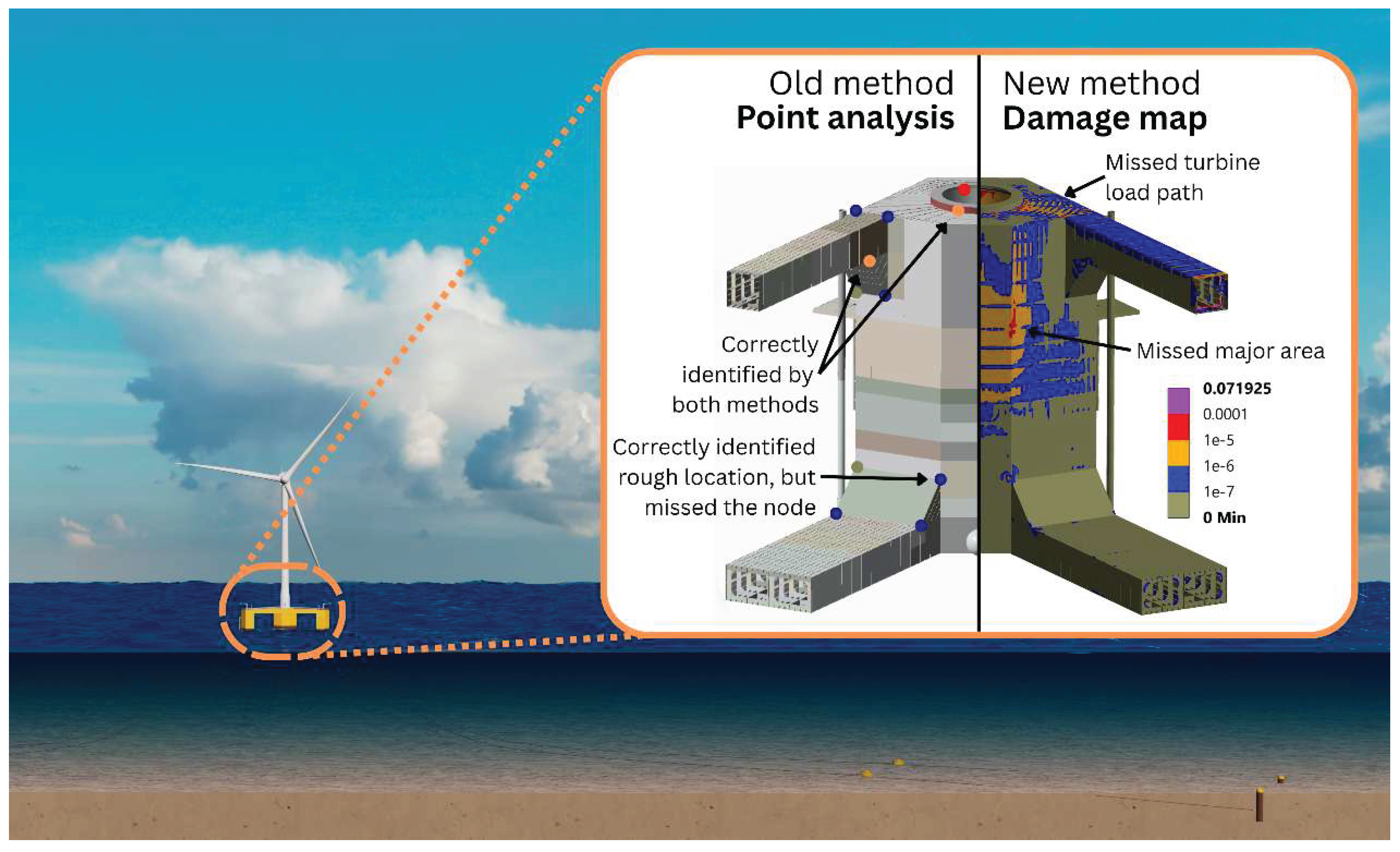
Figure 2. Concept of sub-modelling principle. Left: Global model. Right: local model.

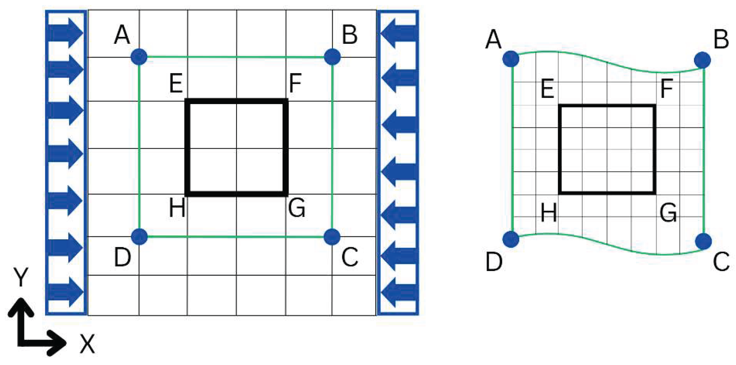
Figure 3. Flowchart for obtaining stress history in this paper.

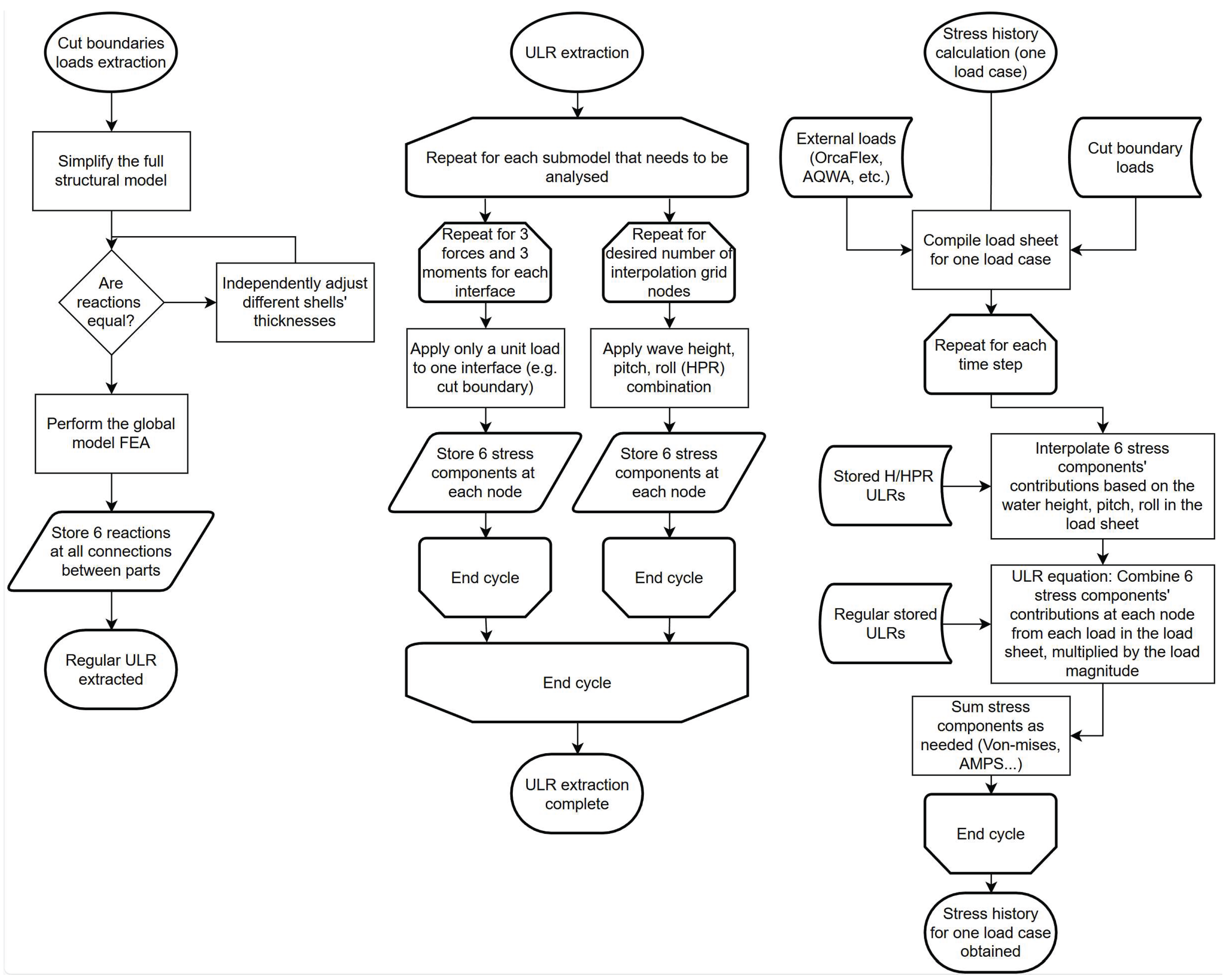
Figure 4. Portal frame problem definition (left) and bending moment diagram (right).

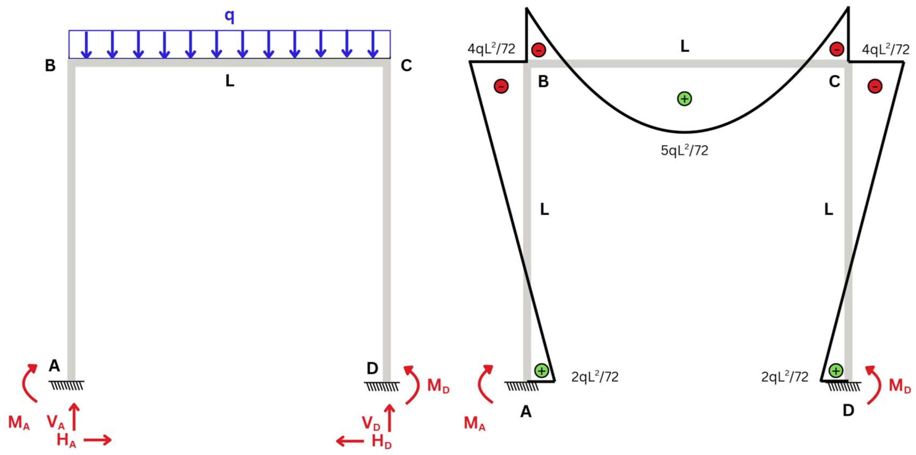
Figure 5. The black vertices of a cube are known data points. Trilinear interpolation proceeds along each orthogonal axis in turn, first reducing the cube to a plane (green), then decreasing the plane to a line (red), and lastly reducing the line to a single point (star). The concept of a mixed interpolation grid is illustrated on the right.

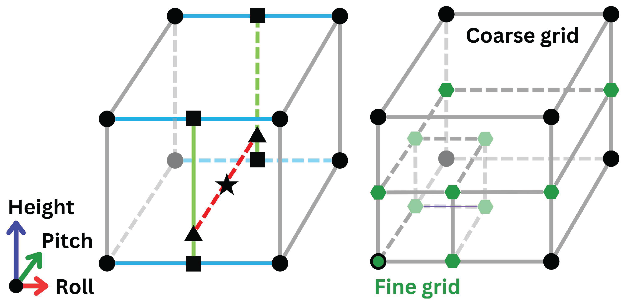
Figure 6. Ways to simplify wave pressure load. The blue line represents the effective water surface.

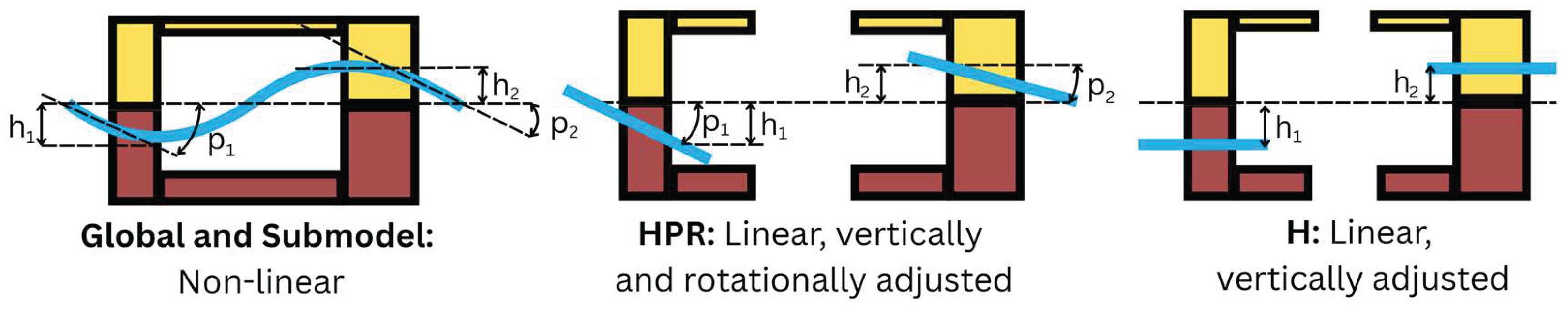
Figure 7. 3D frame element names, control points and submodel boundaries (left) and load case definition (right).

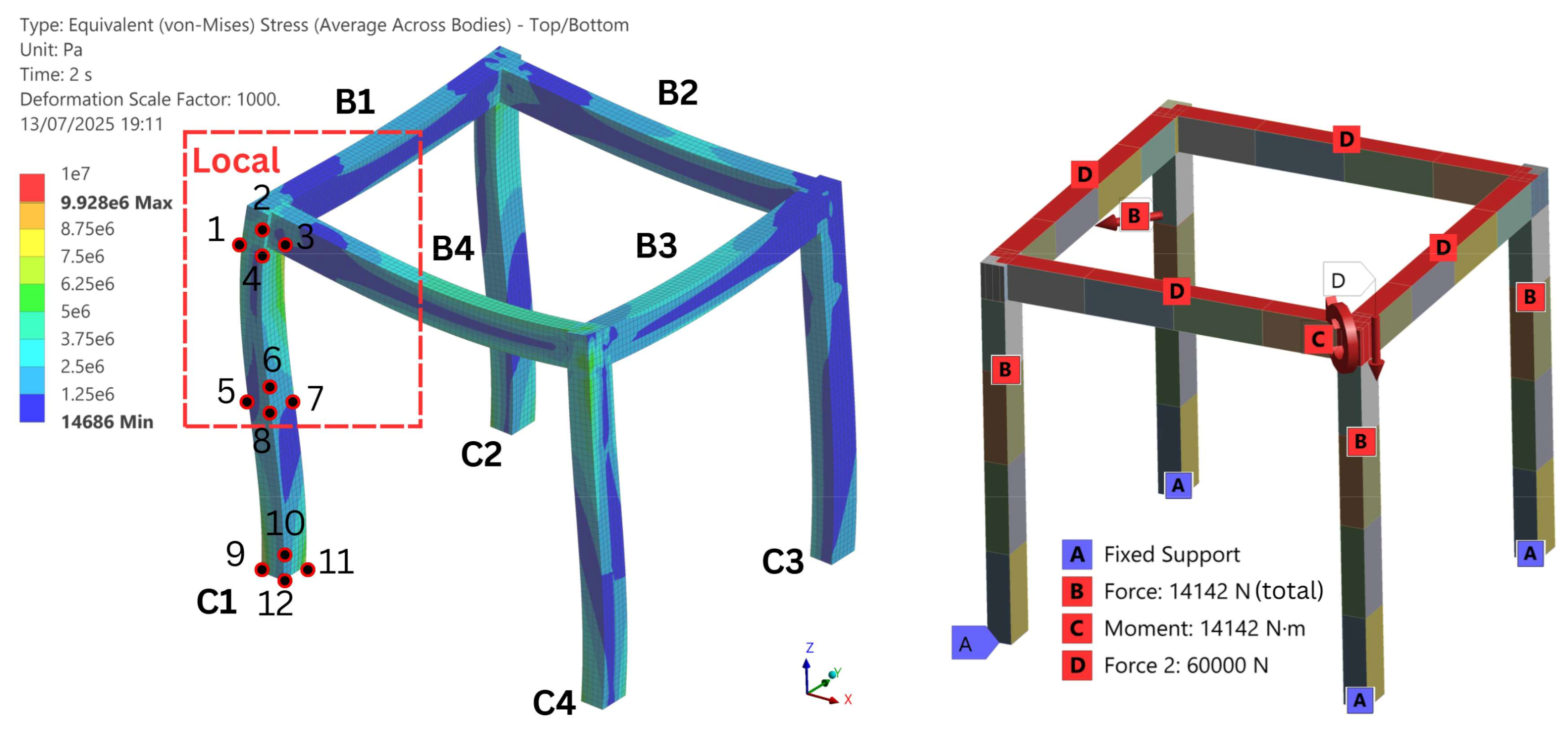
Figure 8. Boundary conditions variations of the local model of a 3D frame structure.

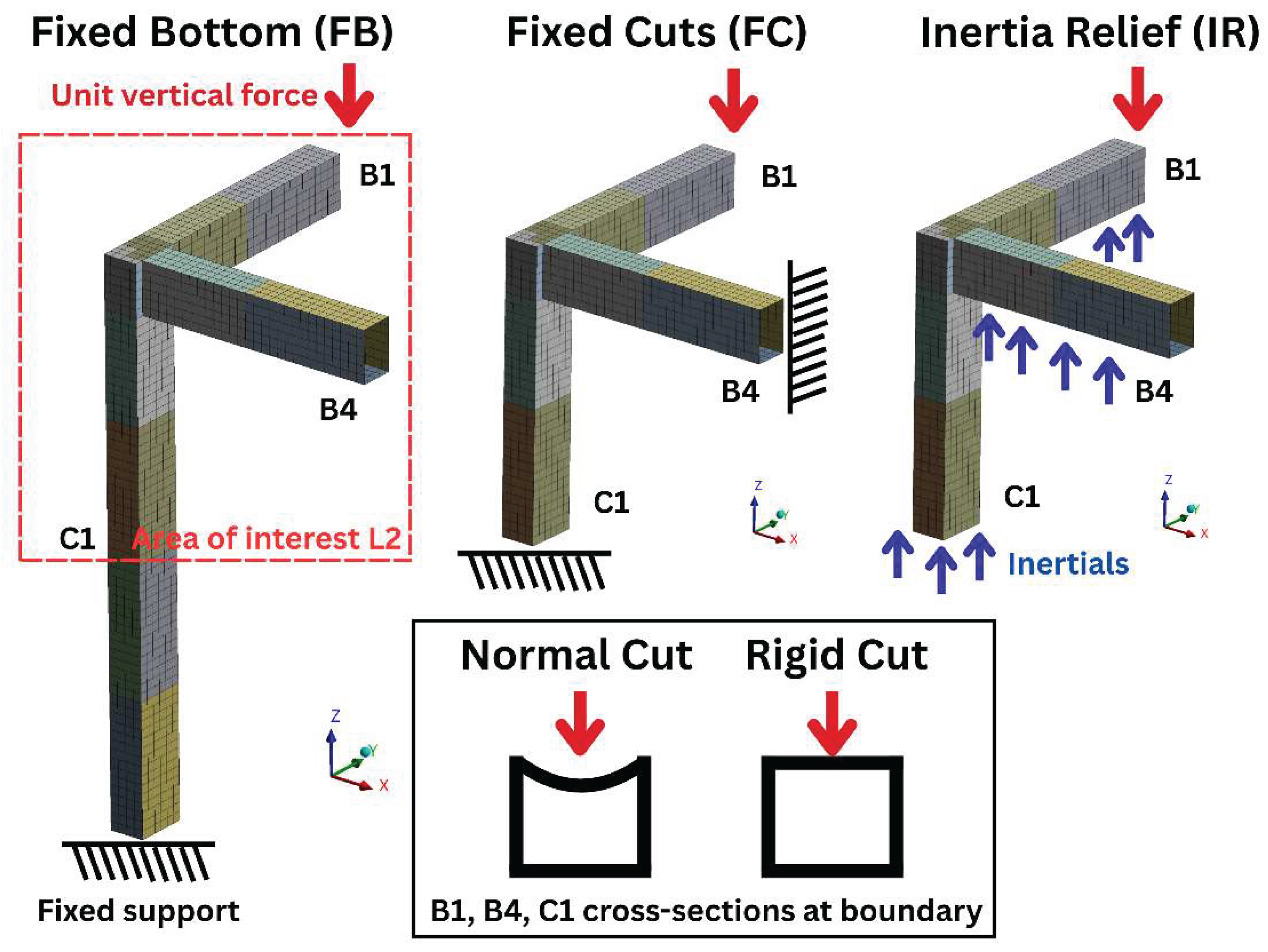
Figure 9. Local model errors relative to the global model.

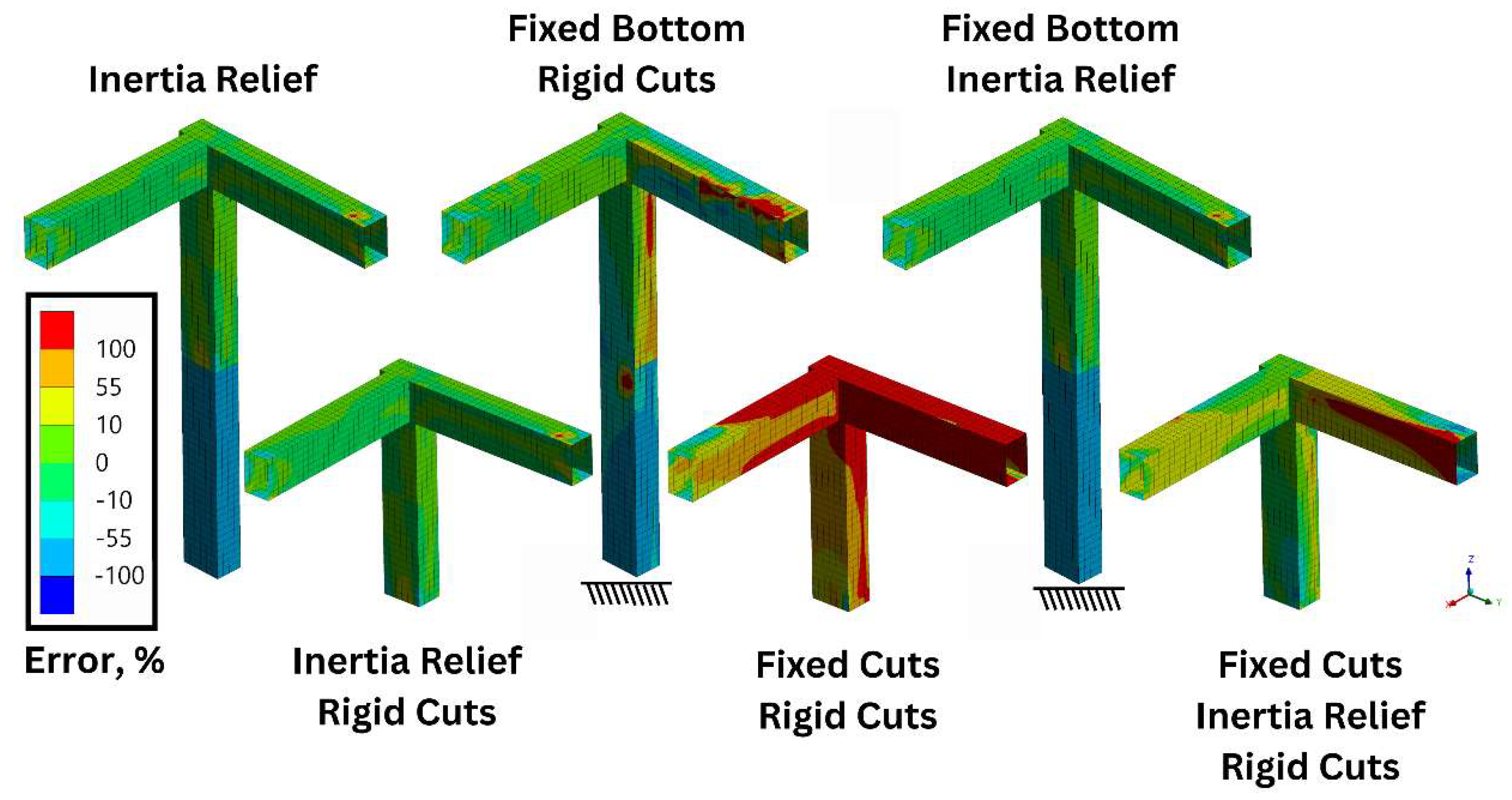
Figure 11. Pressure distributions for different heave, pitch, and roll combinations.

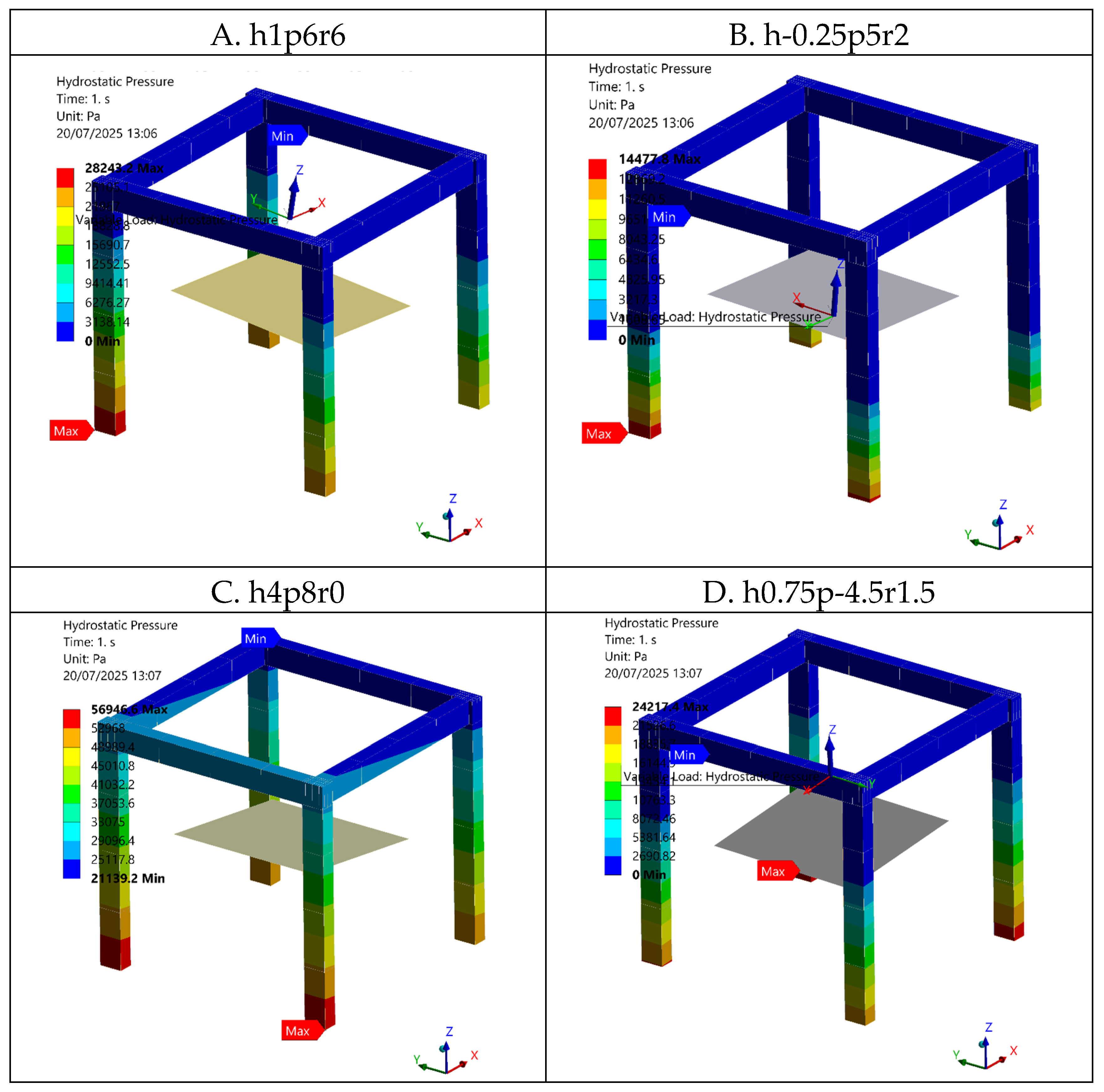
Figure 15. Deformation plots of detailed and simplified model parts on the test rig.

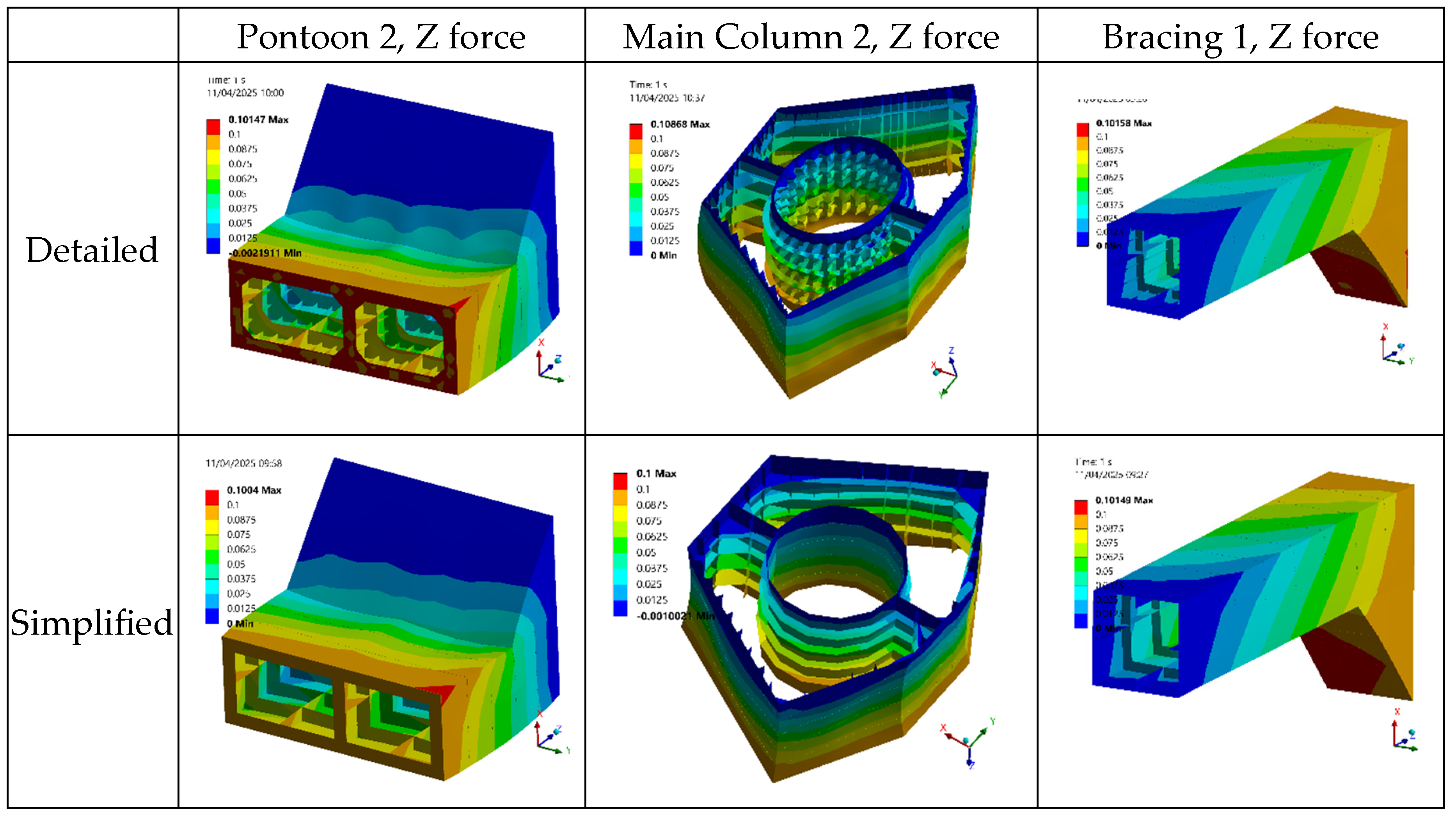
Figure 16. Representative ULRs (deformation exaggerated).

Figure 17. Stress history snapshots obtained via different methods are compared at stress concentrations of the hull.

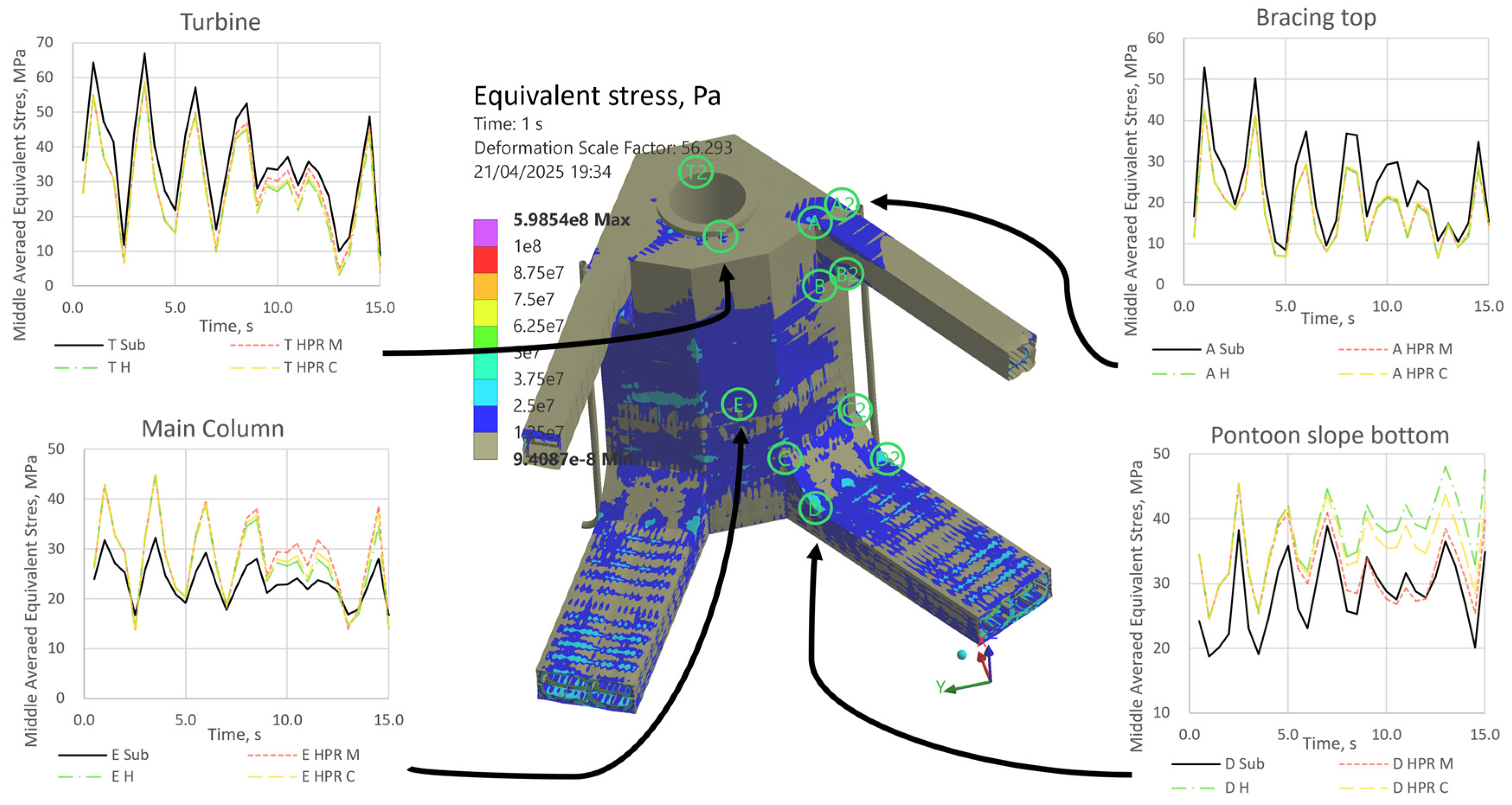
Figure 18. Stress snapshot at 15s time for submodel and 3 ULRs.

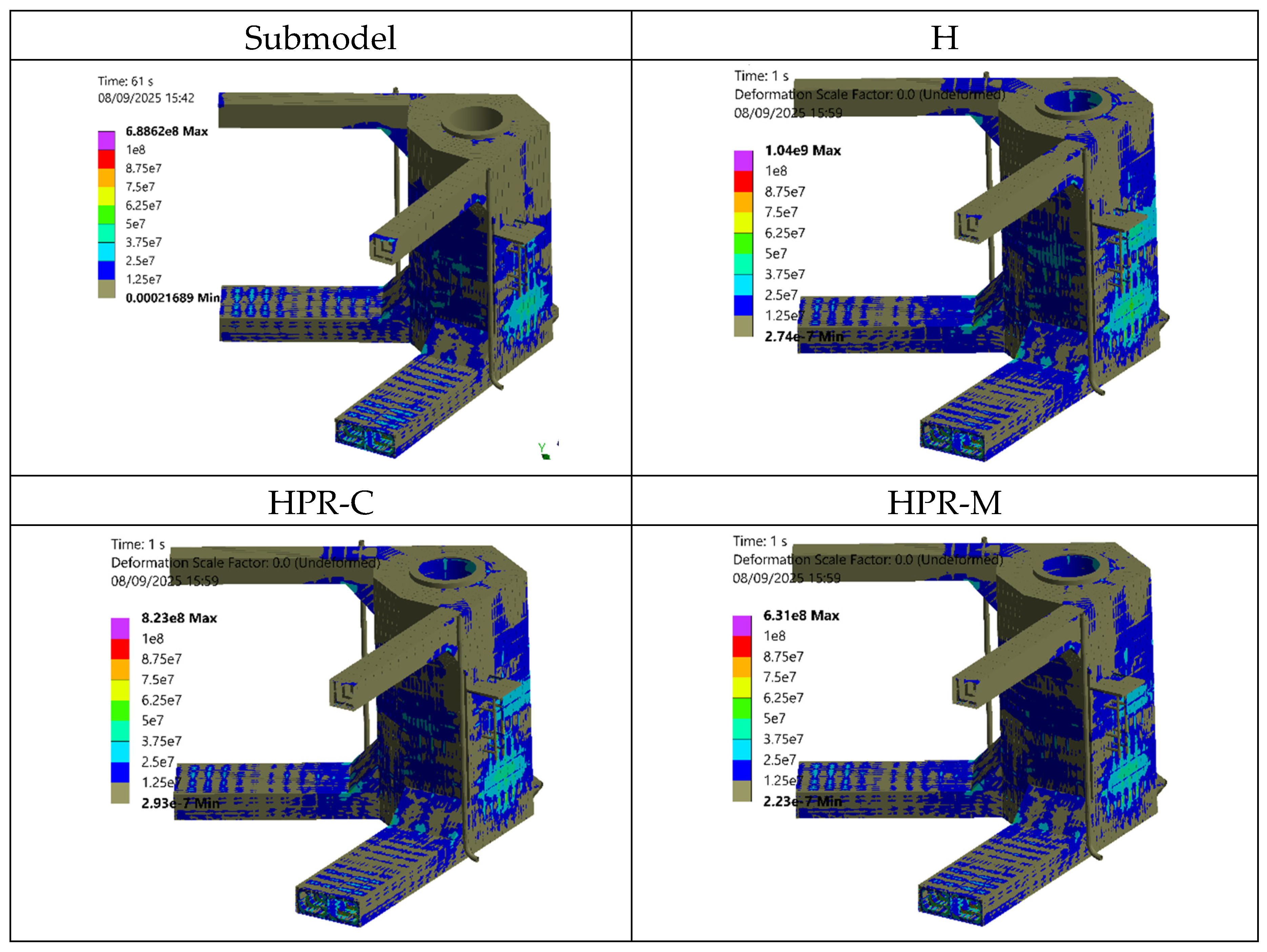
Figure 19. Fatigue damage plots for the three ULR strategies and submodel.

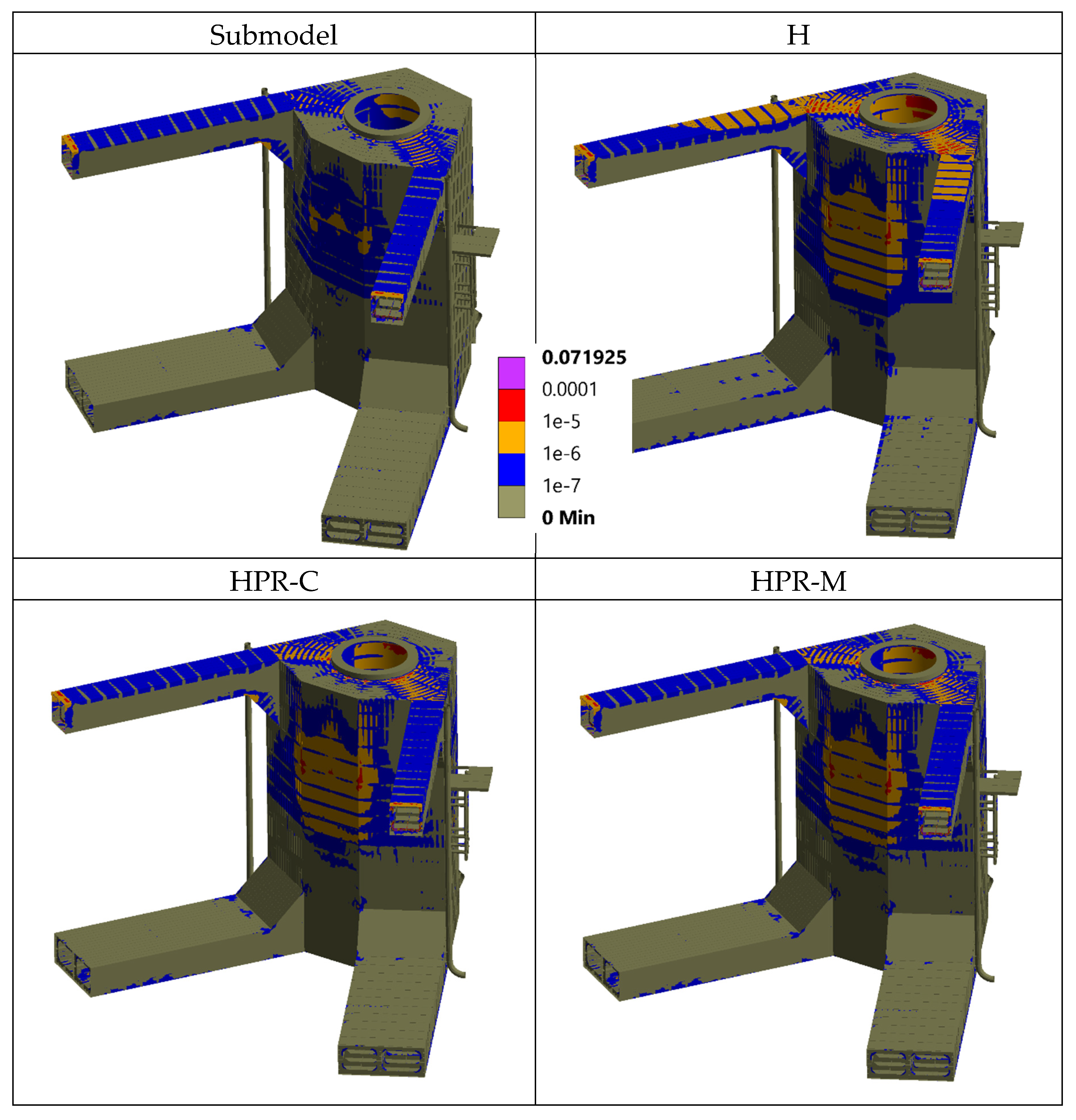
Figure 20. Structures well-suited for the Unit Load Response-Submodelling method application.

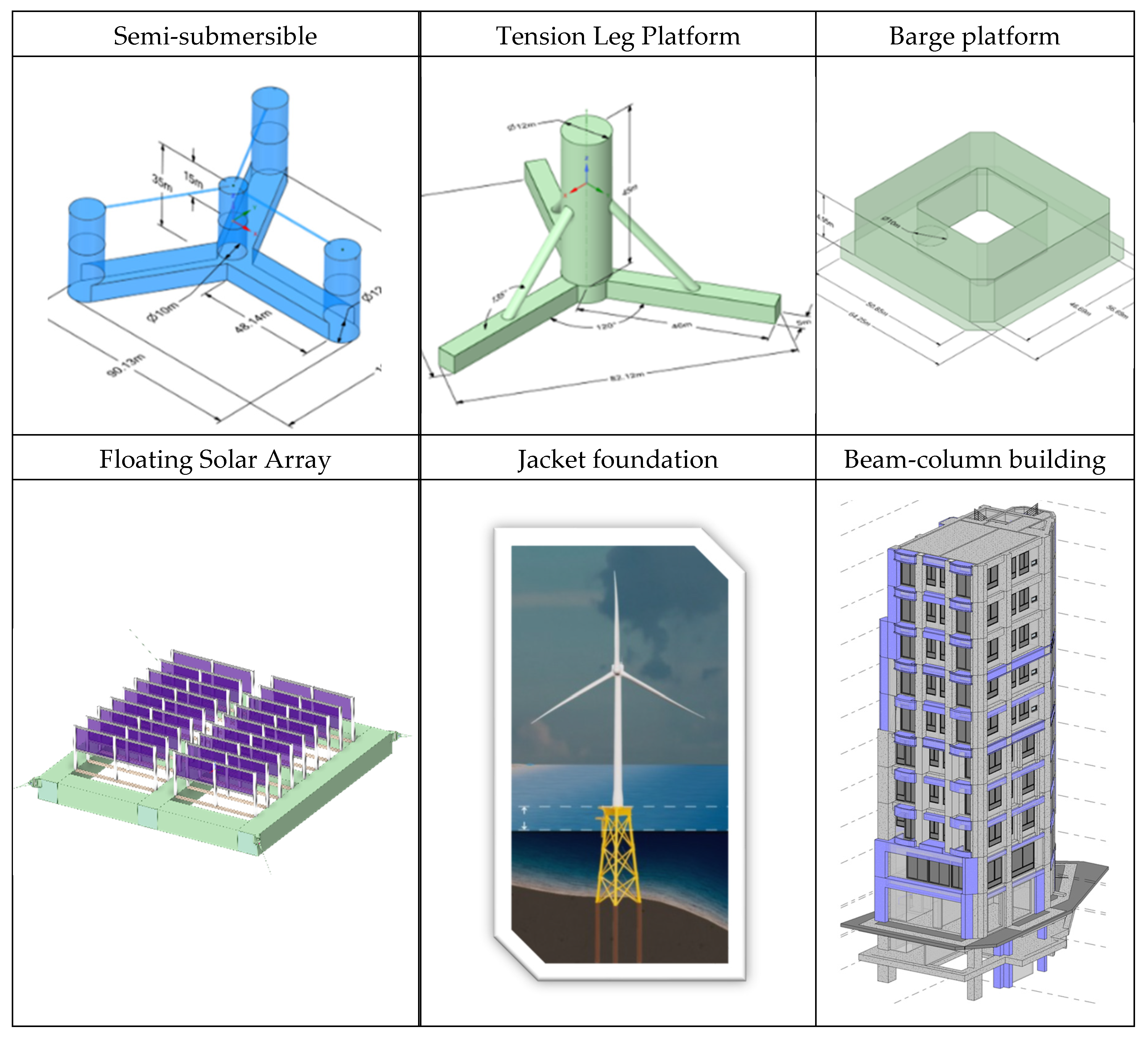
Table 1. Comparison of moment and stress between the analytical solution and various 3D portal frame FE models.

	ANALYTICAL	BEAM B1 2D	SHELL B1 2D	BEAM B1 3D	SHELL B1 3D	BEAM B2 3D	SHELL B2 3D
M_Y	12500	12690	12564	12694	12675	15075	15554
ERROR	0%	1.52%	0.51%	1.55%	1.40%	20.60%	24.43%
∑_XX	8.951	9.088	8.772	9.091	8.860	10.684	10.538
ERROR	0%	1.53%	-2.00%	1.56%	-1.02%	19.36%	17.73%

Table 2. 3D frame ULR and Submodelling error comparison.

AVERAGE ERROR ACROSS TOP NODES	Glob. Shell	Glob. Beam	Local shell, load from global beam	Local shell, load from global shell	Local shell, load from global shell, rigid cut boundary
SUBMODEL	-	4%	23%	4%	4%
ULR	-	4%	13%	2%	2%
AVERAGE ERROR ACROSS 12 NODES	Glob. Shell	Glob. Beam	Local shell, load from global beam	Local shell, load from global shell	Local shell, load from global shell, rigid cut boundary
SUBMODEL	-	-2%	1%	-2%	-1%
ULR	-	-2%	15%	53%	-4%

Table 3. Loads extracted from the shell and beam global models. Red font highlights large discrepancies. Absolute values are used to highlight the relative importance of the loads.

FORCE	BEAM	SHELL	FORCE	BEAM	SHELL	FORCE	BEAM	SHELL	FORCE	BEAM	SHELL
B1_FX	1304.7	1339.2	C1_FX	19783	19805	B4_FX	2021.7	2023.3	B1D_FZ	-7500	-7500
B1_FY	-233.42	-237.3	C1_FY	-4288.2	-4286	B4_FY	247.77	239.9	B4D_FZ	-7500	-7500
B1_FZ	709.56	1007.7	C1_FZ	-3556.9	-3599.3	B4_FZ	4073.3	4051.2	FP_FX	-2500	-2500
B1_MX	165.24	124.63	C1_MX	-18.29	5.6399	B4_MX	564.15	403.44	FP_FY	-2500	-2500
B1_MY	-3282.4	-3226	C1_MY	-698.24	-681.89	B4_MY	-6074	-6277	C1_FX	19783	19805
B1_MZ	1.8803	49.934	C1_MZ	751.21	637.88	B4_MZ	1.3486	-40.4	C1_FY	-4288.2	-4286

Table 4. Accuracy assessment of different boundary conditions for the 3D frame structure. Green colour highlights the mentioned results.

Boundary conditions			Absolute median error, %						Kendallτ-a (excluding boundaries)
Fixed	Inertia relief	Rigid cut	Distributed	Combined	Moment	Combined w/o distr.	Median of 4	Average of 4	Distributed	Combined	Moment	Combined w/o distr.	Median of 4	Average of 4
Bottom	Yes	No	4.89	3.21	0.11	0.51	1.86	25.06	0.94	0.97	1.00	1.00	0.98	0.98
No	Yes	No	4.89	3.21	0.11	0.51	1.86	25.06	0.94	0.97	1.00	1.00	0.98	0.98
No	Yes	Yes	4.89	3.21	0.11	0.51	1.86	25.06	0.94	0.97	1.00	1.00	0.98	0.98
Cut	No	Yes	19.66	12.82	13.61	11.73	13.21	25.95	0.76	0.83	0.85	0.89	0.84	0.83
Bottom	No	Yes	9.18	7.06	40.83	15.23	12.21	62.13	0.92	0.93	0.53	0.84	0.88	0.80
Cut	No	Yes	135.12	70.08	70.15	117.15	93.65	141.44	0.30	0.54	0.77	0.72	0.63	0.58

Table 7. Error in reaction loads of simplified model as compared to the detailed model, by part. Red font highlights large discrepancies, green highlights principal loads of importance.

PART	FX	FY	FZ	MX	MY	MZ
PONT1	-5.6%	-3.6%	-4.6%	3.0%	0.7%	-2.4%
PONT2	0.5%	1.7%	2.1%	-1.9%	-1.3%	-15.2%
MC1	5.5%	-2.7%	-0.8%	-2.6%	0.1%	-0.8%
MC2	9.3%	7.2%	-1.9%	7.6%	0.2%	-31.4%
MC3	0.3%	0.4%	-3.1%	0.5%	0.4%	6.3%
BR1	-3.2%	-10.9%	0.3%	-6.2%	-0.7%	-61.3%
BR2	-2.7%	-2.7%	-9.2%	-2.7%	-2.7%	-288.3%
SC1	-4.7%	-5.1%	7.9%	9.3%	-0.6%	-1.8%
SC2	-3.7%	-3.1%	-14.2%	-6.1%	-4.2%	-4.9%
SC3	7.6%	4.4%	-0.4%	-0.2%	0.1%	10.5%

Table 8. Summary comparison of the three ULR interpolation strategies.

	H	HPR-C	HPR-M
Number of ULRs used	66	570	1411
Average stress error (concentrations)	-4.9%	-3.8%	-4.1%
Median fatigue error (concentrations)	-21.4%	-24.3%	-23.0%
τ-a value of stress spot ranking (all points)	0.428	0.867	0.867
τ-a value of fatigue spot ranking (concentrations)	0.714	0.758	0.758
τ-a value of fatigue spot ranking (all points)	0.709	0.822	0.822

Table 9. Expected fatigue calculation time for HPR-C in this case study using an Intel i9-13900HX (2.20 GHz) processor.

STAGE	PRESENT METHOD	CLASSIC SUBMODELLING
Time-domain global load simulations (e.g., OrcaFlex)	1 h per bin × 184 ≈ 184 h
AQWA pressure field simulations on the hull	0.5 h per bin × 184 ≈ 92 h
Simplified model simulation for cut-boundary loads	3 h per bin × 184 ≈ 552 h
Local model simulations	0.4 h per bin × 184 ≈ 74 h	60 h per bin × 184 × 3 submodels ≈ 33120 h
Stress history extraction	3 h per bin × 184 × 3 submodels ≈ 1656 h	0.15 h per bin × 184 × 3 submodels ≈ 83 h
Rainflow counting and fatigue damage calculation	0.2 h per bin × 184 × 3 submodels ≈ 110 h
Total computational time	2668 hours ≈ 111 days	34141 hours ≈ 1423 days
Relative computational time	7.8%, 12.8 times less	100%

Disclaimer/Publisher’s Note: The statements, opinions and data contained in all publications are solely those of the individual author(s) and contributor(s) and not of MDPI and/or the editor(s). MDPI and/or the editor(s) disclaim responsibility for any injury to people or property resulting from any ideas, methods, instructions or products referred to in the content.

© 2025 by the authors. Licensee MDPI, Basel, Switzerland. This article is an open access article distributed under the terms and conditions of the Creative Commons Attribution (CC BY) license (http://creativecommons.org/licenses/by/4.0/).

Copyright: This open access article is published under a Creative Commons CC BY 4.0 license, which permit the free download, distribution, and reuse, provided that the author and preprint are cited in any reuse.