
Submitted:
25 November 2025
Posted:
26 November 2025
You are already at the latest version
Abstract
Understanding resonance and frequency behavior is fundamental in engineering acoustics and in technology-supported music-learning environments. This work presents an Educational Acoustics Audio System (EAAS) designed as a sensor-based hardware–software toolkit that enables experiential learning of acoustic resonance through listening, spectrogram visualization, and analytical modeling. The system integrates a bass-reflex loudspeaker with interchangeable vent configurations, a microphone-based sensing module, automated spatial sampling, and a MATLAB interface for generating logarithmic sweeps, recording responses, and computing high-resolution spectrograms. The instructional design is grounded in the Educational Acoustics Conceptual Framework (EACF), originally proposed by the authors, which structures learning through concrete, graphical, and abstract levels. Learners first explore perceptual changes in low-frequency amplification, then interpret time–frequency patterns using spectrograms, and finally compute Helmholtz-based resonance frequencies based on physical parameters. Experimental measurements collected at multiple microphone distances reveal stable resonance peaks at approximately 546 Hz (full vent) and 265 Hz (half vent), alongside consistent amplitude differences between vent configurations. By integrating auditory perception, sensor-based acquisition, and mathematical modeling in a unified and low-cost system, the EAAS provides an effective technological platform for hands-on exploration of resonance and frequency response. This approach strengthens conceptual understanding in engineering acoustics while supporting its application in related educational contexts.
Keywords:
educational acoustics
; resonance frequency
; spectrogram visualization
; hardware–software educational toolkit
1. Introduction
In recent years, the field of acoustics has evolved beyond its traditional scientific boundaries, becoming a key component in technological innovation, human–machine interaction, and educational practice. Advances in digital signal processing, artificial intelligence, and low-cost sensing technologies have expanded the possibilities for acoustic experimentation and learning. Acoustics is often regarded as a graduate-only branch of engineering. This perception arises from the highly complex mathematical models involved and the multidisciplinary nature of the field [1,2]. Although it is possible to introduce acoustics at the undergraduate level, several challenges hinder its integration. Usually, undergraduate academic programs related to this discipline are already full of mandatory courses, leaving acoustics, in the best-case scenario, as an elective-only course [1,3,4]. As a result, recent graduates tend to have a polarized profile: they either have a solid formation in the field or lack formal exposure to it altogether.
This uneven educational preparation implies a growing challenge for local industries, where the demand for acoustic expertise is steadily increasing. Especially within mechanical, electrical and civil engineering, as well as physics or even computer science applications [2,3]. This gap between educational practices and professional requirements therefore represents an opportunity to enhance current curricula, especially in programs that already contain acoustics-related content.
Among engineering majors, mechanical engineering offers perchance the most direct pathway into acoustics. Courses such as mechanical vibrations, machine dynamics and advanced manufacturing naturally intersect with acoustic principles and can serve as effective entry points into the field [4]. Integrating acoustic topics within these courses not only helps address the educational gap but also broadens students’ perspectives on how acoustics influence design, innovation, and system behavior. Strengthening the presence of acoustics in engineering education thus becomes both a strategic and necessary step.
One of the principal barriers to integrating acoustic into undergraduate education lies in the specialized equipment typically required for accurate signal measurement and analysis [4]. While this is a valid concern across most acoustic-related subfields, certain core concepts can nonetheless be explored effectively using common laboratory tools and software. Within this context, audio stands out as one of the most accessible domains of acoustics. Its direct connection to physical phenomena facilitates comprehension of otherwise abstract concepts, making audio experimentation a powerful pedagogical resource [5]. When employed strategically, audio experimentation becomes more than a convenient entry point; it emerges as a robust teaching method that effectively bridges theory and perception. Moreover, music acoustics represents a natural application domain for teaching resonance and frequency behavior, as musicians and learners rely on auditory perception and spectral cues to understand timbre, instrument response, and sound-production processes.
Through guided experimentation and basic signal analysis, students can create immediate perceptual links to theoretical concepts; for instance, frequency response, reverberation or resonance [5]. These activities also introduce learners to basic, yet essential analysis tools, particularly spectrograms. By visualizing sound in the time-frequency domain, spectrograms allow students to interpret signals that would otherwise be difficult to analyze by ear alone. This dual auditory-visual approach reinforces comprehension and equips students with transferable analytical skills [5,6]. In music-learning environments, these same auditory–visual strategies are widely employed to help learners identify spectral patterns, understand resonance peaks in sound-producing systems, and develop perceptual skills essential for timbre recognition and pitch stability. Collectively, the literature and current industrial trends suggest that incorporating acoustics more systematically into undergraduate engineering curricula helps form professionals better equipped for increasingly sophisticated technological challenges.
In contrast, previous educational efforts to introduce acoustics at the undergraduate level have generally taken two forms: elective courses with strong technical orientation and practical assignments centered around signal analysis [7,8]. Both approaches have proven to yield substantial results in bringing acoustics closer to students. However, they frequently fall short in cultivating the analytical depth required to link physical phenomena with mathematical models, a connection that is critical for a profound and enduring understanding of the discipline.
To contextualize the status of educational acoustics, several existing educational kits were examined as state-of-the-art references. In general, these kits can be categorized into two distinct groups: highly specialized professional systems, which are cost-prohibitive and complex for entry-level instruction, and simplified demonstration kits, which lack the analytical depth required for comprehensive study. For example, the Polytec VibroGo kit provides a sophisticated platform that supports wireless acoustic analysis; however, its high cost and steep learning curve limit its suitability for introductory education [9]. In contrast, kits such as the Simple Resonance Kit by United Scientific, the Student Kiy by 3B Scientific, and the Acoustic Resonance Apparatus by HomeScienceTools offer accessible demonstrations of fundamental principles, such as resonance [10,11,12]. Despite their pedagogical value, these tools remain mainly illustrative and are not designed to support advanced or inquiry-based learning environments. This connection is especially relevant for music-technology education, where accessible sensing tools and spectrogram-based analysis are increasingly used to support training in instrument acoustics, sound design, and performance evaluation.
To address this limitation, the present work proposes the development of the EAAS Toolkit based on acoustic baffle design parameters to demonstrate frequency response and resonance. This toolkit enables students to modify design variables and observe their effects both audibly and visually through spectrogram analysis. The novelty of this work lies in adapting and integrating an Educational Acoustics Conceptual Framework (EACF) as the pedagogical foundation to teach acoustic-engineering concepts, particularly resonance and resonance frequency, through hands-on experimentation. By situating acoustics within the broader context of mechatronic education, the study bridges theoretical and experiential learning, linking sensing, actuation, and control through sound-based activities. In addition, because resonance behavior and time–frequency interpretation are essential analytical skills in both engineering acoustics and music-learning environments, the EAAS provides a learning approach that reflects the auditory and visual reasoning used in instrument acoustics and sound-production analysis. This approach strengthens students’ conceptual understanding of dynamic systems and highlights how educational acoustics can support transferable analytical skills relevant to both engineering and music-technology contexts.
2. Educational Acoustics Conceptual Framework
To achieve the construction of the EACF, it is essential to position the student as an active participant in the learning process. Drawing from already established educational frameworks in engineering, it is possible to design an adaptation specifically for acoustics. As previously noted, this framework should be built upon closely related disciplines, particularly mechanical engineering. The framework presented in [13] for mechatronics is especially relevant, as it is both related to acoustics and shares a similar multidisciplinary nature, thereby allowing a more direct transfer of its learning methodology. According to this model, students require four reference perspectives to comprehend abstract concepts: process, application, scenario and artifact (see Figure 1).
Within the domain of acoustics, the process perspective corresponds to the fundamental physical concepts of the field. The application perspective identifies the technological areas in which these principles can be employed. The scenario perspective further specifies these applications by contextualizing them in specific physical environments, where they are intended to operate. Lastly, the artifact perspective integrates the previous dimensions into the design and creation of acoustic components, resulting in the materialization of abstract concepts.
The purpose of implementing these perspectives is to guide students through three progressive levels of learning: concrete, graphic and abstract [13]. At the concrete level, students are introduced to the discipline through direct interaction with the artifacts, which allows them to physically engage with the phenomena under study [5,13]. Once familiar with the equipment and having collected initial data, students transition to the graphic level, where they connect the observed physical phenomena with symbolic representations. This progression culminates in the abstract level, where learners synthesize these connections into a deeper understanding of the fundamental concepts of the field. By structuring learning in this way, the framework supports a gradual yet comprehensive development of knowledge, enabling students to bridge practical experience with theoretical abstraction.
3. Implementation of the Educational Acoustics Audio System
The Educational Acoustics Audio System (EAAS) is composed of a bass-reflex loudspeaker and a microphone configuration. The loudspeaker baffle must be constructed or modified to include a single circular port. Additionally, customized 3D-printed plastic caps and foam gaskets are required to regulate the vent opening. The EAAS hardware setup consists of a laptop, a condenser microphone, an audio interface with phantom power, a bass-orientated passive loudspeaker, an adapted bass-reflex baffle, and the 3D printed caps and gaskets. The approximate cost of the complete setup is $400 USD. However, given the relatively simple nature of the box modifications, the system can be assembled using repurposed equipment.
The primary objective of the EAAS is to promote experimental learning in frequency response and resonance by enabling adjustments to the system’s resonance frequency and observing the corresponding changes in its output. To properly operate the system, the aforementioned hardware must be complemented by software, specifically a programming environment for signal generation and analysis, and a DAW (Digital Audio Workstation) for audio recording. Figure 2 illustrates the proposed setup.
The mechanical design of the EAAS was developed through an iterative process that began with hand-drawn conceptual sketches defining the placement path of the loudspeaker and microphone, controlled by a linear actuator. These initial sketches were used to establish the geometry of the system, identify spatial constraints, and determine component interactions. Based on these early layouts, a parametric 3D model was created in CAD software, allowing precise definition of dimensions, tolerances, and mounting interfaces for each component. The design was refined through several iterations to optimize structural rigidity, ensure proper alignment between the rail and microphone carriage, and provide secure housing for the electronics. The final CAD model, shown in Figure 3, served as the basis for fabricating the structural frame. Additionally, the vent caps and foam gaskets were modeled (as show in Figure 4) in order to 3D-print and laser cut them respectively. Both CAD models were crucial for the integration of the mechanical and electronic subsystems into a cohesive measurement platform.
3.1. The EAAS Hardware
The EAAS generates, reproduces and records sound files to obtain the baffle’s frequency response. For this purpose, .wav files are recommended, as their lack of compression ensures higher fidelity. The minimum hardware requirements for the controlling laptop are 4 GB of RAM and a 1 GHz CPU. The condenser microphone and audio interface must support a minimum sampling rate of 40 kHz to satisfy Nyquist’s theorem and prevent aliasing across the full range of human hearing (20 Hz – 20 kHz) [14].
Regarding the 3D-printed vent caps and gaskeys, any variation in vent length or effective depth may be evaluated; however, it is advisable to begin with the full-vent and half-vent configurations. All vent configurations should maintain a circular geometry to facilitate compatibility with the Helmholtz-resonator model used throughout the experiment.
Figure 5 shows the complete EAAS hardware setup. The bass-reflex loudspeaker is positioned at one end of the structure, with the interchangeable vent mounted directly on the front baffle. A condenser microphone is installed on a carriage that moves along an aluminum rail driven by a linear actuator, enabling automated spatial sampling of the acoustic field. Two limit switches define the actuator’s travel range, ensuring repeatable and safe operation during each measurement cycle. The electronics enclosure houses the microcontroller, motor driver, and power circuitry required for automated microphone positioning. This arrangement allows the system to perform controlled and consistent measurements of the loudspeaker’s acoustic response.
3.2. The EAAS Software
The EAAS employs MATLAB to generate, reproduce, and analyze the test signals used to characterize the loudspeaker’s acoustic response. MATLAB is used to synthesize excitation signals, including logarithmic frequency sweeps and Gaussian noise, which are exported as uncompressed .wav files. These files are then imported into Reaper (DAW), where simultaneous playback and recording ensure that the captured microphone response remains time-aligned with the original excitation signal, thereby facilitating accurate post-processing and deconvolution. After each recording session, the resulting audio file is exported from the DAW and processed in MATLAB to compute spectrograms, extract resonance behavior, and evaluate the baffle’s frequency response.
To simplify this workflow and reduce the need for manual scripting, a dedicated graphical user interface (GUI) was developed in MATLAB App Designer. As shown in Figure 6, the EAAS Toolkit interface is organized into three functional sections. The Signal Generation panel includes a dual-slider for selecting the sweep’s start and end frequencies within the human hearing frequency range (20 Hz kHz), a field for specifying sweep duration, and Gen and Play buttons for generating and previewing excitation signals. The Distance Setting panel allows the user to define the microphone position along the linear actuator using a centimeter-based slider, with the Set button communicating the selected position to the Arduino-controlled motor system. Finally, the Spectrogram panel visualizes the processed acoustic response and includes an Export button for saving the resulting plot. This integrated interface enables students to conduct the measurement procedure efficiently while reinforcing the connection between signal generation, automated acquisition, and spectral analysis.
3.3. Signal Generation
Although the system can operate with any signal type, a full frequency sweep is recommended for didactic purposes. However, the main interest lies within the sub-bass to lower midrange (20 – 500 Hz); since, this frequency interval refers to what a bass-reflex baffle should amplify [15,16]. The duration of the sweep is not critical, though approximately ten seconds is optimal to achieve a smooth transition. Importantly, the signal must be generated using the system’s sampling frequency (minimum 40 kHz) and exported as a .wav file to prevent compression-related distortion.
3.4. Resonance Frequency Calculation
In a separate MATLAB script, the baffle’s resonance frequency is calculated by approximating the system as a Helmholtz resonator, as supported by existing literature on bass-reflex loudspeakers [17]. This requires measuring the baffle’s dimensions and determining its internal volume, vent cross-sectional area, and vent depth. The resonance frequency is then computed using Equation (1) for all vent configurations.
where f represents the system’s resonance frequency, c sound’s speed, A the vent’s cross-sectional area, V the system’s internal volume and the vent’s depth.
3.5. Response Recordings
The DAW must be configured to match the previously defined sampling rate; otherwise, discrepancies will arise between the recording and the input signal. Once configured, the test signal is imported into one track, and secondary tracks are created and armed for recording. To focus the measurement on the baffle’s resonance, the loudspeaker should be positioned at any distance around one meter from the microphone [18]. The user first records the unmodified vent response, followed by a second recording with one of the 3D-printed caps mounted on the system. Each response must be recorded on its own track. The user must try to identify response differences attributable to vent modifications, representing the concrete level of learning. In addition to synthetic excitation signals, the EAAS is also compatible with musical inputs: students may record and analyze isolated instrumental tones, scales, or short musical phrases, allowing the system to be adapted for studying resonance, timbre evolution, and spectral behavior under realistic music-acoustics conditions.
3.6. Response’s Spectogram Analysis
The response recordings are subsequently imported into MATLAB, where the spectrogram function in the Audio Toolbox is used to generate the raw signal’s spectrogram. Learners are then tasked with interpreting the spectrogram and predicting what changes are expected on the system response signals based on the calculated resonance frequencies, which aligns with the graphical level. Finally, the spectrograms of the system responses are plotted and contrasted, enabling the learner to establish relationships between the baffle’s design parameters, resonance frequency, and frequency response. This final stage corresponds to the abstract level of learning.
4. Instructional Design
The instructional design is structured around the Educational Acoustics Conceptual Framework (EACF), incorporating its four perspectives. Specifically, students engage with resonance (process) in the context of audio (application), employing the EAAS (scenario) with the modified bass-reflex loudspeaker (artifact). The learning experience is organized into three progressive stages, corresponding to the concrete, graphical and abstract levels of the EACF. Within this framework, students modify the loudspeaker’s design parameters, collect and analyze acoustic responses, predict changes and interpret these responses using spectrograms.
To strengthen conceptual understanding, the full trajectory through the three EACF levels is repeated for three different microphone–loudspeaker distances: m, m, and m. This enables students to compare how spatial positioning affects the captured acoustic field and the resulting frequency-response and resonance patterns.
Practice: Frequency sweep analysis
This exercise is designed to facilitate students’ understanding of frequency response as a fundamental tool in audio system design. The EACF is applied in the following manner: students first explore the audible effects of resonance at the concrete level, then visualize amplitude variations using spectrograms at the graphical level, and finally relate these observations to the underlying physical and mathematical principles at the abstract level. By repeating this process at m, m, and m, learners gain practical insight into distance-dependent acoustic phenomena such as attenuation, spatial dispersion, and energy distribution in the bass-reflex system.
Concrete level At the concrete level, students engage in direct interaction with the experimental setup:
- Students position the loudspeaker and microphone in alignment, ensuring both devices face one another.
- Students initiate recording in the DAW and carefully listen the system’s response.
- A 3D-printed cap is placed on the loudspeaker’s vent.
- Students create a new track in the DAW and record the modified response while attentively listening.
- Steps 3-4 may be repeated depending on the number of vent configurations under investigation. In this case, we have a full-vent and a half-vent.
Figure 7 shows the three microphone positions used in the experiment illustrating the near-field, mid-range and far-field configurations employed to analyze distance-dependent variations in the bass-reflex system.
Graphical level At the graphical level, students translate their concrete experiences into symbolic representations:
- The instructor generates the spectrogram of the original signal used in the concrete level.
- The instructor provides guidance on interpreting spectrograms.
- Students predict how the system’s response spectrogram will vary based on their auditory observations. Ideally, students identify regions they anticipate will exhibit amplification due to resonance.
Abstract level At the abstract level, students integrate symbolic representations with theoretical understanding, focusing on the concept of resonance. Resonance occurs near a system’s natural frequency, and the presence of damping typically shifts the resonance toward lower frequencies. Bass-reflex systems are commonly modeled as Helmholtz resonators, for which the resonance frequency can be calculated using Equation (1). The students’ tasks at this level are as follows:
- Compute the resonance frequency of the system for all vent configurations.
- Adjust the original predictions regarding the system’s acoustic output based on the calculated resonance frequencies.
- Generate spectrograms for all vent configuration responses and compare them with the initial predictions.
This structured progression, from direct experimentation to symbolic interpretations and finally to theoretical integration, ensures that students develop a comprehensive understanding of the relationships between design parameters, resonance frequency and frequency response in audio equipment.
5. Results
The spectrogram of the excitation signal used in the EAAS, corresponding to a logarithmic sweep from 20Hz to 20 kHz over 10 seconds is shown in Figure 8. The red curve indicates the increasing sweep frequency, while the color scale represents signal amplitude, with warmer colors denoting higher energy. This reference spectrogram is used to compare and analyze the loudspeaker’s measured acoustic response.
A single metric was employed to evaluate the performance of the EAAS: the average amplitude across the bass-reflex loudspeaker’s operational frequency range. As mentioned previously, this type of loudspeaker is expected to amplify frequencies within the sub-bass to lower midrange spectrum (20 – 500Hz). By calculating the average amplitude and expressing it on a decibel (dB) scale, it is possible to quantitatively assess the relative amplification provided by different vent configurations.
5.1. EAAS Average Amplitude Assessment
Using MATLAB’s spectrogram analysis tool, the average amplitude within the specified frequency window was computed for all recorded system responses. Additionally, a recording of the laboratory’s ambient noise was imported into MATLAB and subjected to the same analytical procedure to establish a baseline reference. Amplitude values were subsequently converted to the dB scale using Equation (2). The results were plotted, and mean amplitudes were determined (see Figure 11, Figure 14, Figure 17). This approach enables a comparative evaluation of the system’s responses relative to one another and to the ambient noise within the target frequency range.
Where represents the signal’s amplitude in dB, the signal’s original amplitude and the reference signal’s average amplitude.
The Bass-Reflex resonance frequencies were computed with Equation (1) according to each vent configuration. These calculations are presented on Equations (3) and (4).
where the subscripts and refer to the full and half vent configurations, respectively.
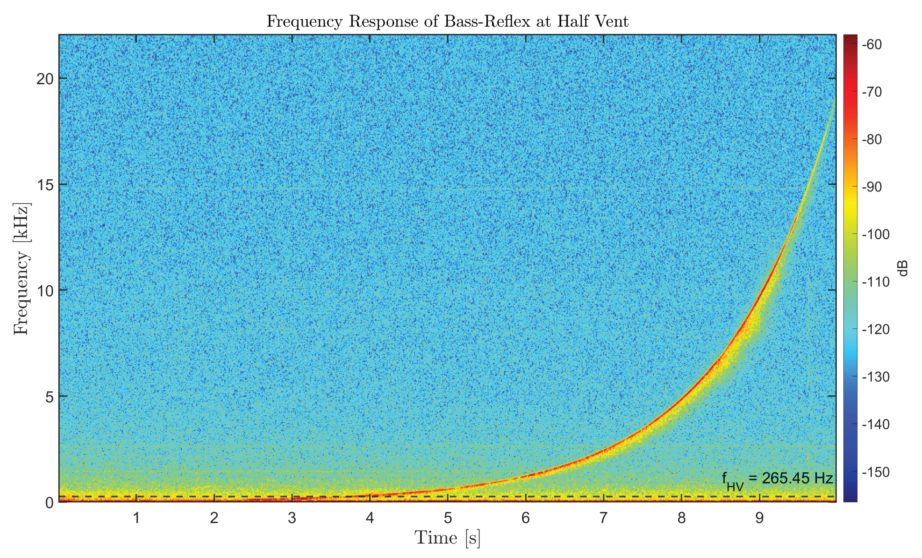
Figure 9, Figure 10 and Figure 11 compare the acoustic response of the bass-reflex loudspeaker under the full-vent and half-vent configurations. The spectrograms (Figure 9 and Figure 10) show the recorded sweep from 20 Hz to 20 kHz, with the resonance frequency clearly visible in each case. The averaged amplitude curves in the 20–500 Hz band (Figure 11) reveal that the full-vent configuration exhibits a mean amplitude of dB, whereas the half-vent configuration yields dB. This difference of dB corresponds to an increase of approximately in amplitude for the full vent relative to the half vent. Furthermore, both configurations exceed the ambient noise level, with the full vent measuring about 86% above ambient and the half vent about 33% above ambient. These results demonstrate the EAAS’s ability to distinguish vent-dependent variations in low-frequency acoustic performance.
Figure 9.
Full Vent Bass-Reflex Spectogram at 0.3m.
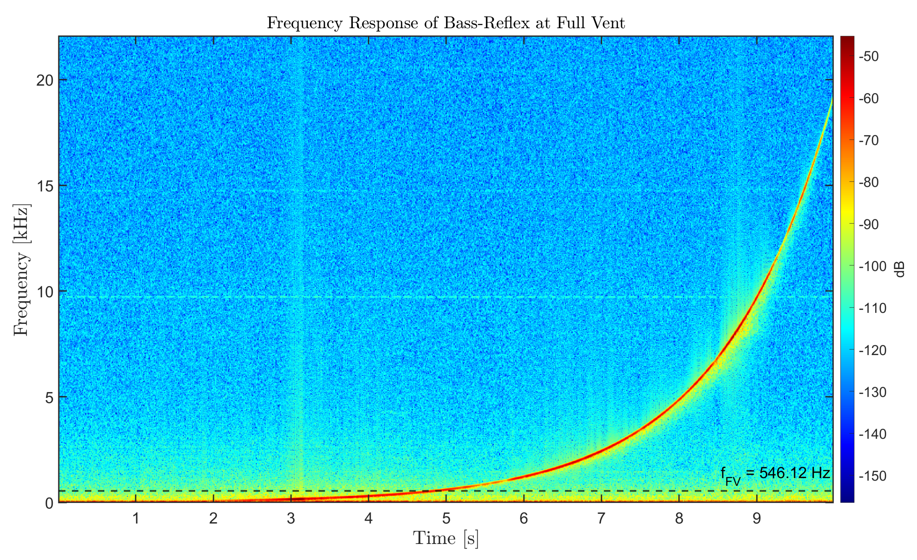
Figure 10.
Half Vent Bass-Reflex Spectogram at 0.3m.
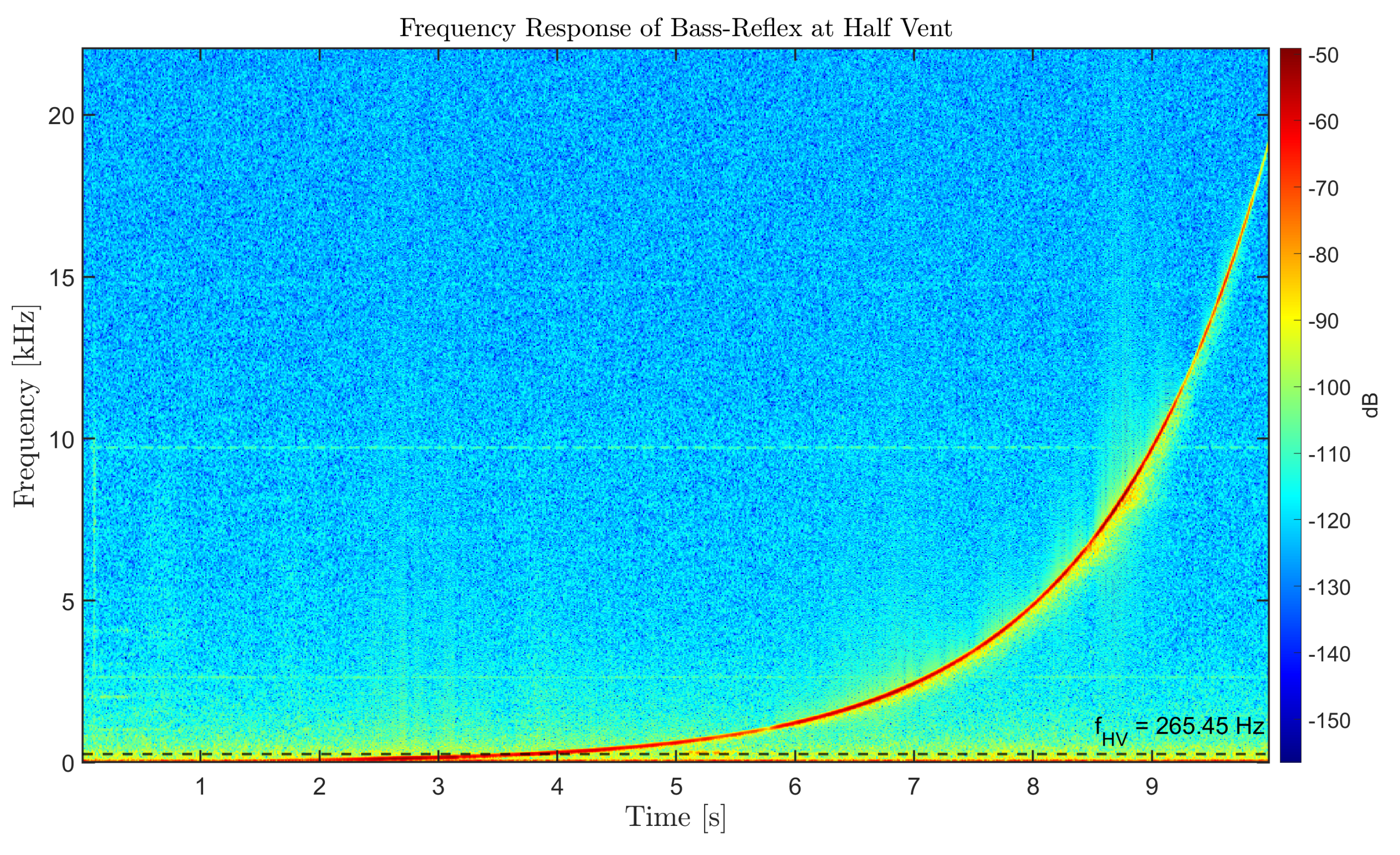
Figure 11.
Bass-Reflex Amplitude Comparison at 0.3m.
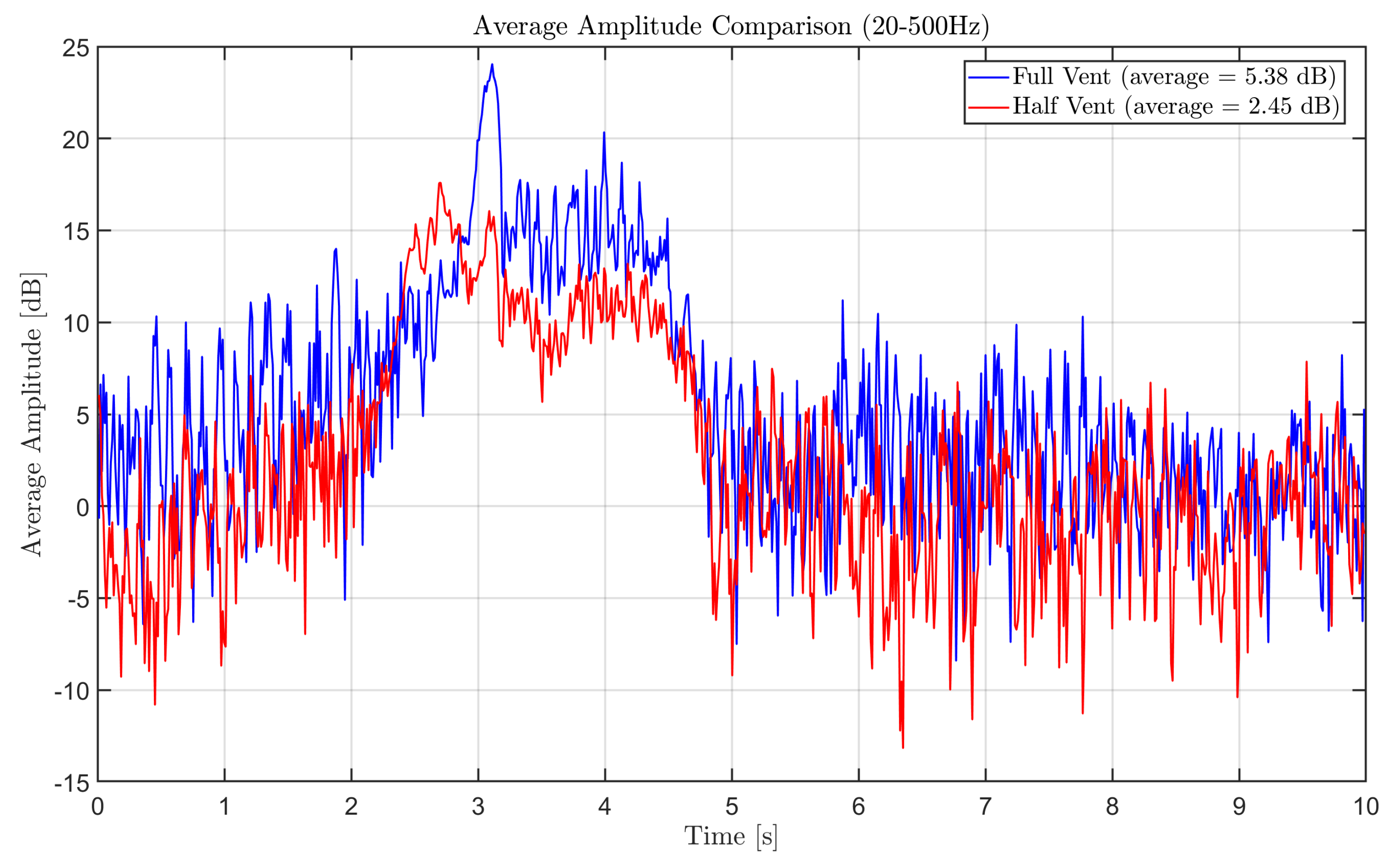
Figure 12, Figure 13 and Figure 14 present the spectrograms and average amplitude comparison for the full-vent and half-vent configurations at m. The averaged amplitude curves in the 20-500 Hz range (Figure 14) indicate mean values of dB for the full vent and dB for the half vent, meaning the full-vent response is approximately 28% higher in amplitude. Both configurations remain above the ambient noise level, confirming that the EAAS effectively captures vent-dependent differences at mid-range distance.
Figure 12.
Full Vent Bass-Reflex Spectogram at 0.7m.
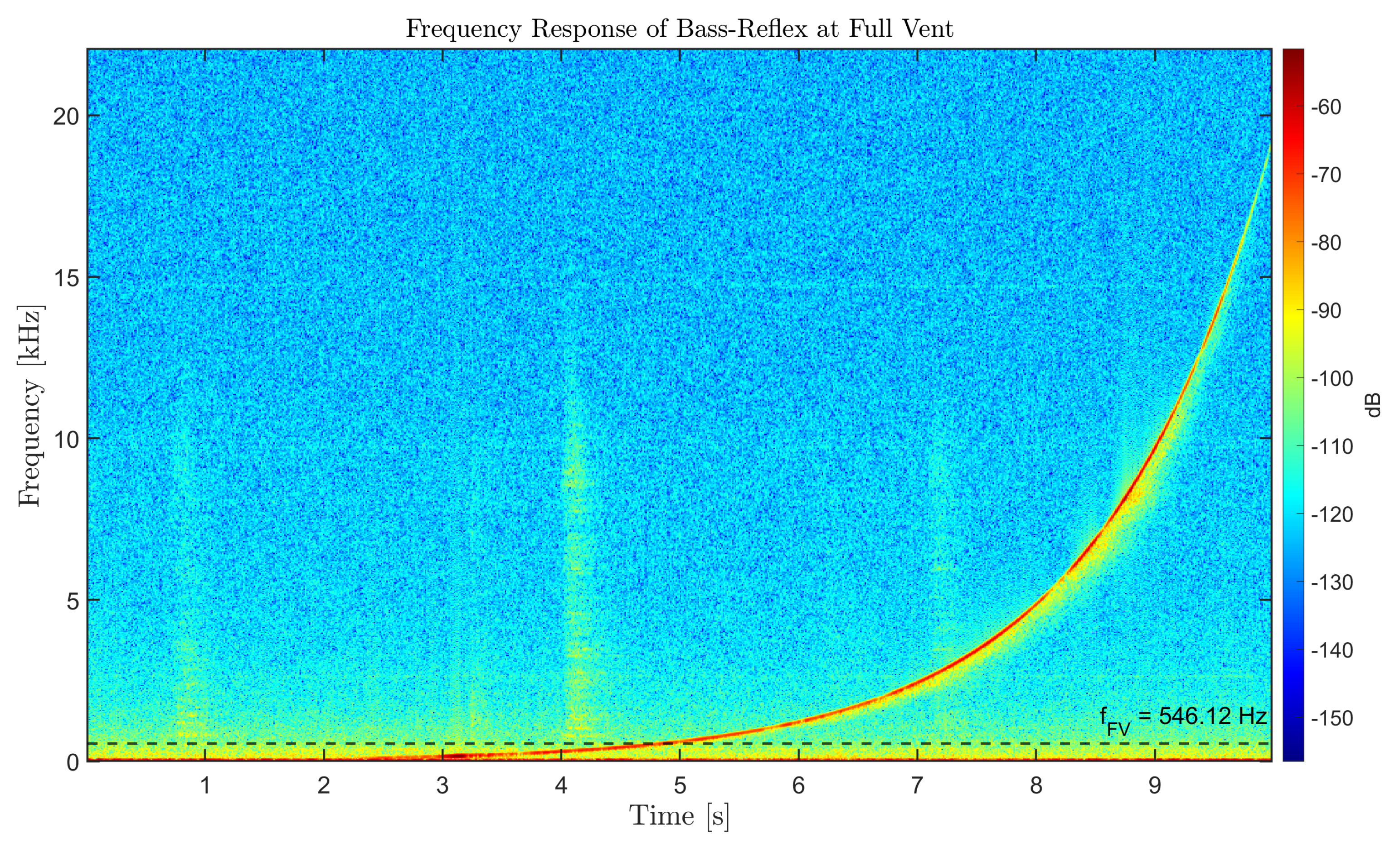
Figure 13.
Half Vent Bass-Reflex Spectogram at 0.7m.
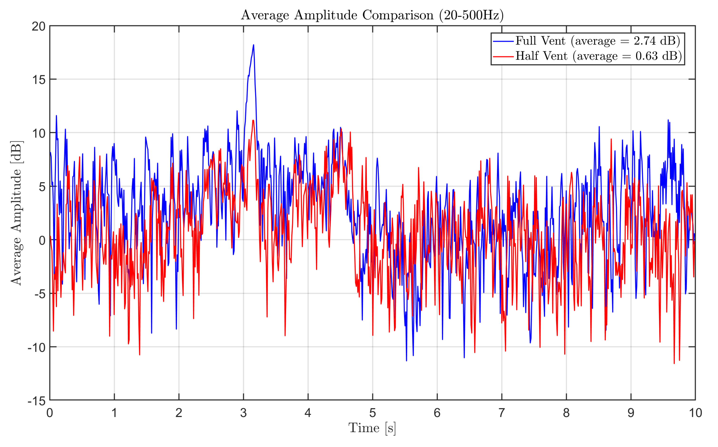
Figure 14.
Bass-Reflex Amplitude Comparison at 0.7m.
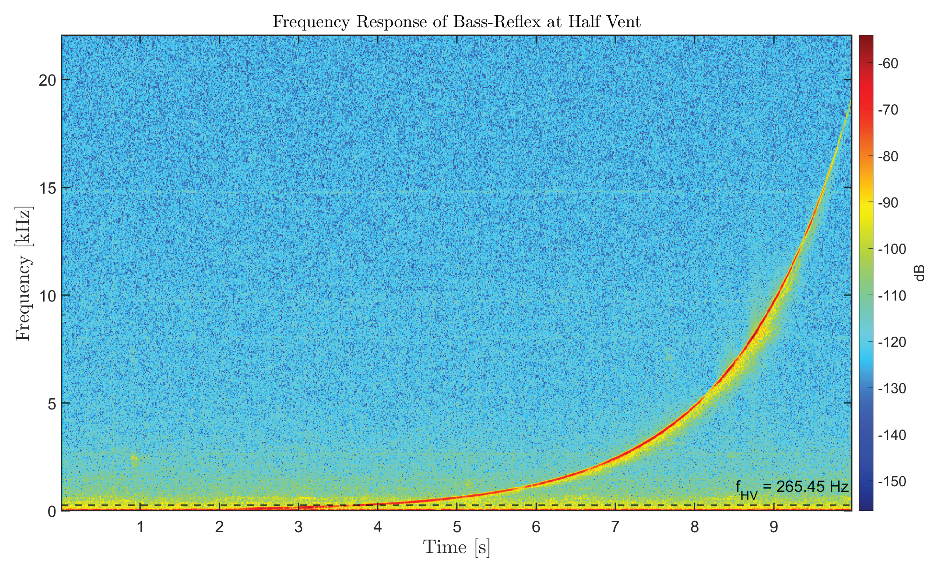
Figure 15, Figure 16 and Figure 17 show the spectrograms and average amplitude comparison for the full-vent and half-vent configurations at a 1 m microphone distance. The averaged amplitude curves in the 20-500 Hz band (Figure 17) yield mean values of dB for the full vent and – dB for the half vent, indicating that the full-vent configuration is approximately 23% higher in amplitude. The full vent remains slightly above the ambient noise level, while the half vent falls below it, demonstrating the reduced low-frequency energy captured at far-field distance.
A comparison of the three measurement distances ( m, m, and m) shows a progressive reduction in low-frequency amplitude as the microphone is positioned farther from the loudspeaker, while the resonance frequencies remain consistent across all distances. For the full-vent configuration, the resonance peak appears at approximately 546 Hz, whereas for the half-vent configuration, the resonance shifts to around 265 Hz, as expected from the change in effective vent depth. At m, the full vent reaches a mean amplitude of dB, about 40% higher than the half vent ( dB). At m, amplitudes decrease but the full vent ( dB) remains 28% stronger than the half vent ( dB), with both resonance frequencies clearly visible in the spectrograms. At m, attenuation becomes more pronounced: the full vent measures dB, still 23% higher than the half vent (- dB), and both resonance peaks, 546 Hz and 265 Hz, remain identifiable despite the reduced signal energy. These results demonstrate that increasing distance reduces measured amplitude, but the resonance behaviour of each vent configuration remains stable, confirming the reliability of the EAAS measurements across varying spatial conditions.
Figure 17.
Bass-Reflex Amplitude Comparison at 1m.

6. Discussion
Modern engineering industry is increasingly demanding acoustic solutions across a wide range of applications; however, acoustics remain predominantly considered a specialization-only field. While it is true that the discipline employs complex mathematical models and exhibits an intrinsically multidisciplinary nature, undergraduate students can acquire foundational knowledge around it [1,2,3]. Such learning experiences not only complement the existing curriculum but may also inspire students to pursue further specialization in acoustics.
Most state-of-the-art developments in acoustic education target graduate-level students or address acoustics concepts primarily at a technical level [7,8]. In contrast, this work emphasizes the introduction of undergraduate students to a more conceptual and abstract approach to studying and understanding acoustics. Specifically, it adapts the educational engineering methodology presented in [13] to the acoustics domain. The proposed EACF supports the teaching–learning process through a three-level pedagogical structure and specifically addresses resonance and resonance-frequency concepts within the context of audio design applications. By promoting engagement through controlled experimentation and structured analysis, the methodology fosters both conceptual understanding and potential interest in advanced study.
Accordingly, the EAAS seeks to integrate acoustic principles into undergraduate engineering curricula by embedding them within existing courses such as mechanical vibrations. The system enables comparative assessments of audio equipment to determine their suitability for specific frequency ranges using both qualitative listening and quantitative spectrogram-based analysis. Furthermore, the EAAS can be calibrated to provide results in standardized dB measurements, ensuring accurate and reproducible evaluations aligned with established engineering practices. The experimental results presented in this work, showing stable resonance frequencies across all measurement distances and consistent vent-dependent response differences, validate the EAAS as a reliable sensing platform for educational use.
Although the EAAS Toolkit is applied in the context of engineering education, its underlying principles directly intersect with the objectives of music-technology learning environments. Spectrogram-based analysis, resonance identification, and frequency-response interpretation are central tools not only in audio engineering but also in music acoustics, instrument design, and auditory-perception training. The ability to visualize and quantify resonance behavior supports foundational skills used in music learning—such as understanding timbre formation, recognizing frequency-dependent amplification, and interpreting the spectral behavior of sound-producing systems. Consequently, the EAAS contributes pedagogically relevant sensing technology that can be adapted for music-learning scenarios, providing a bridge between engineering acoustics and music-acoustics education.
Author Contributions
Conceptualization, D.C.-T. and L.F.L.-V.; methodology, D.C.-T. and L.F.L.-V.; software, D.C.-T. and R.I.L.-G.; validation, D.C.-T., J.A.L. and R.I.L.-G.; formal analysis, D.C.-T. and M.E.M.-R.; investigation, D.C.-T., R.I.L.-G. and M.E.M.-R.; resources, L.F.L.-V. and M.A.C.-M.; data curation, D.C.-T., J.A.L. and R.I.L.-G.; writing—original draft preparation, D.C.-T.; writing—review and editing, L.F.L.-V., J.A.L. and M.A.C.-M.; visualization, D.C.-T. and R.I.L.-G.; supervision, L.F.L.-V.; project administration, L.F.L.-V. and M.A.C.-M.; funding acquisition, M.E.M.-R. and M.A.C.-M. All authors have read and agreed to the published version of the manuscript.
Funding
This research received no external funding.
Institutional Review Board Statement
Not applicable.
Informed Consent Statement
Not applicable.
Data Availability Statement
The data presented in this study are available on request from the corresponding author.
Acknowledgments
During the preparation of this manuscript, the authors used ChatGPT [19] for the purposes of language refinement, text restructuring, and improving clarity in the presentation of methods and results. The authors reviewed, validated, and edited all generated content and take full responsibility for the final version of this publication.
Conflicts of Interest
The authors declare no conflicts of interest.
Abbreviations
The following abbreviations are used in this manuscript:
| EA | Educational Acoustics |
| EACF | Educational Acoustics Conceptual Framework |
| EAAS | Educational Acoustics Audio System |
| DAW | Digital Audio Workstation |
| dB | Decibels |
| Hz | Hertz |
| FFT | Fast Fourier Transform |
| GUI | Graphical User Interface |
| CAD | Computer-Aided Design |
| CPU | Central Processing Unit |
| GB | Gigabyte |
| RAM | Random Access Memory |
| WAV | Waveform Audio File Format |
References
- Prasad, M.G. Integrating acoustics into mechanical engineering education. J. Acoust. Soc. Am. 1999, 106, 1–2. [Google Scholar] [CrossRef]
- Institute of Acoustics. Innovations in Acoustics 2020, 1st ed.; The Institute of Acoustics: Milton Keynes, UK, 2020; pp. 1–40. [Google Scholar]
- National Academies of Sciences, Engineering, and Medicine. Ocean Acoustics Education and Expertise, 1st ed.; National Academies Press: Washington, DC, USA, 2025; pp. 75–88. [Google Scholar]
- Prasad, M.G. Acoustics in mechanical engineering undergraduate core courses: Challenges and opportunities. J. Acoust. Soc. Am. 2005, 117, 1–2. [Google Scholar] [CrossRef]
- Ronsse, L.; Cheenne, D.J.; Kaddatz, S. Using your ears: A novel way to teach acoustics. J. Acoust. Soc. Am. 2013, 19, 1–2. [Google Scholar]
- Almallah, N.; Al-Quzwini, M. Introducing spectral analysis to undergraduate engineering students. In Proceedings of the Future of Engineering Education 2024 Annual Conference & Exposition, Portland, OH, USA, 23–26 June 2024. [Google Scholar]
- Gazengel, B.; Ayrault, C. Two examples of education in acoustics for undergraduate and young postgraduate students. In Proceedings of the Acoustics 2012 Nantes Conference, Nantes, France, 23–27 April 2012. [Google Scholar]
- Anderson, M. (Western Reserve University, Cleveland, OH, USA); Berezovsky, J. (Western Reserve University, Cleveland, OH, USA). Advanced undergraduate acoustics experiment. Unpublished work.
- Polytec (Polytec Inc. Irvine, CA). Polytec Education program. Unpublished work.
- HomeScienceTools. Available online: https://www.homesciencetools.com/product/sound-measurement-kit/?srsltid=AfmBOoov7L3tY6B6b3FA_Q272fcrXs9fn_G5bahaT9Vud5cdz2P5Euhz (accessed on 20 October 2025).
- UnitedScientific. Available online: https://www.unitedsci.com/education/physics/simple-resonance-kit.html (accessed on 20 October 2025).
- 3B Scientific. Available online: https://www.3bscientific.com/gb/student-kit-acoustics-1000816-u8440012-3b-scientific,p_780_8254.html (accessed on 20 October 2025).
- Guerrero-Osuna, H.A.; Nava-Pintor, J.A.; Olvera-Olvera, C.A.; Ibarra-Pérez, T.; Carrasco-Navarro, R.; Luque-Vega, L.F. Educational Mechatronics Training System Based on Computer Vision for Mobile Robot. Sustainability 2023, 15, 1386. [Google Scholar] [CrossRef]
- Ozgur, A. (Stanford University, Stanford, CA, USA). Lectures 9-10: Sampling Theorem. Unpublished work.
- Teach Me Audio. Available online: https://www.teachmeaudio.com/mixing/techniques/audio-spectrum (accessed on 15 September 2025).
- Speaker Decision. Available online: https://speakerdecision.com/blog/Seven-Frequency-Bands-of-Audio-Spectrum (accessed on 15 September 2025).
- Deshler, N. (University of California Berkeley, Berkeley, CA, USA). The Helmholtz Resonator. Unpublished work.
- Biering, H. (Brüel & Kjœr, Nærum, DK). Measurement of Loudspeaker and Microphone Performance using Dual Channel FFT-Analysis. Unpublished work.
- OpenAI. ChatGPT (GPT-5.1); OpenAI: San Francisco, CA, USA, 2025; Available online: https://chat.openai.com (accessed on 15 November 2025).
Figure 1.
The Educational Acoustics Coneptual Framework Perspectives.
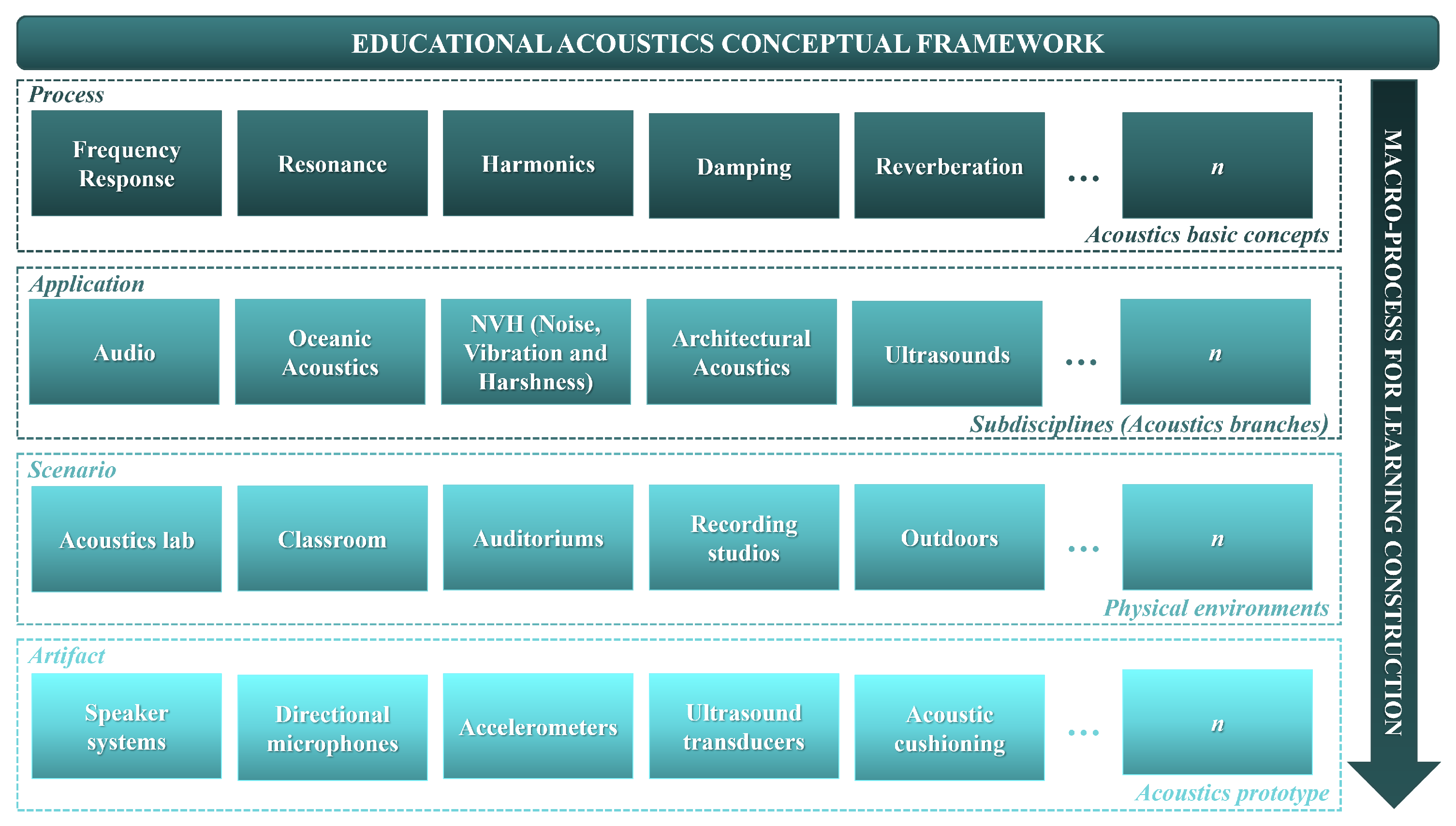
Figure 2.
Proposed system: Educational Acoustics Audio System.
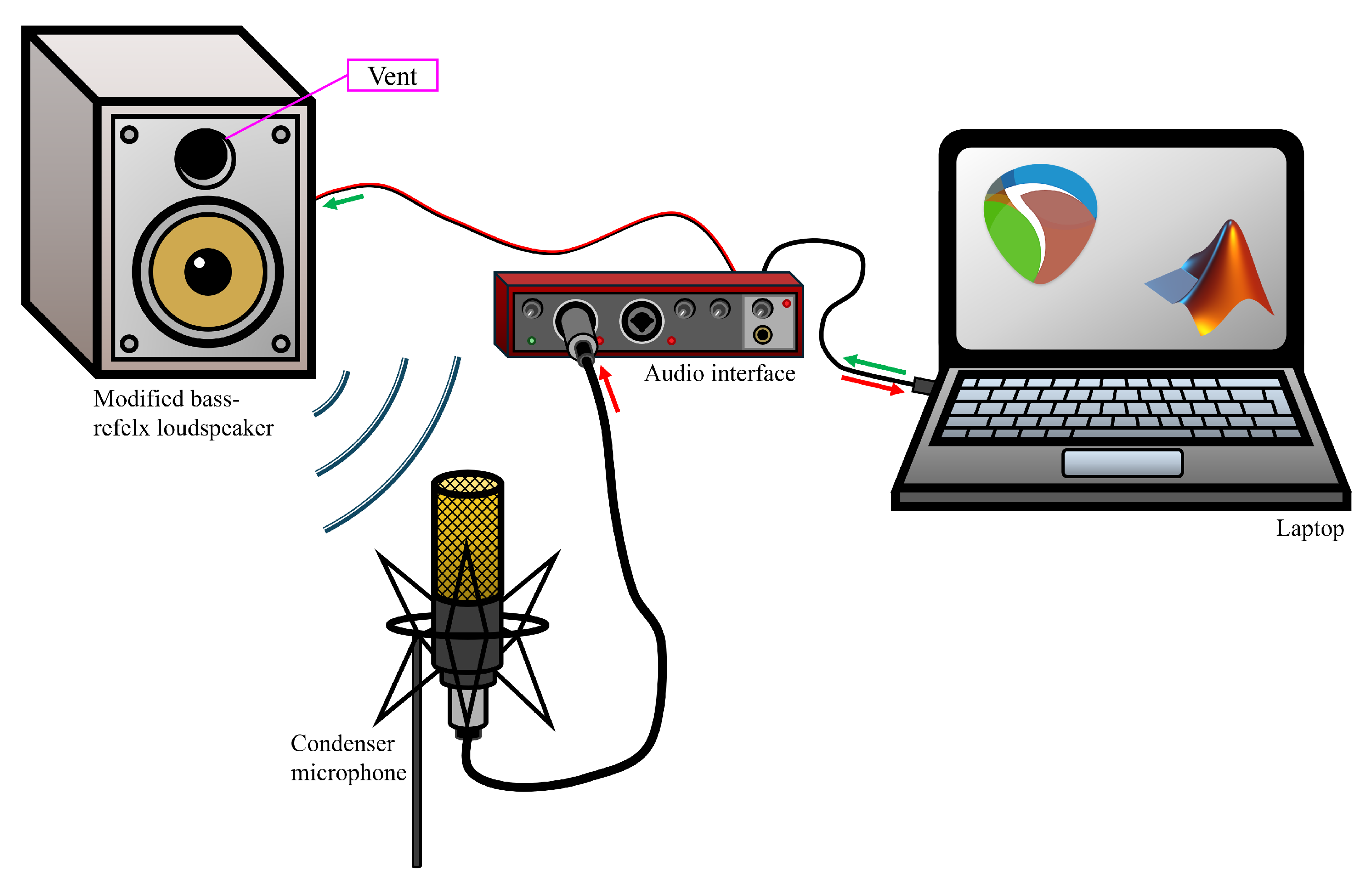
Figure 3.
CAD model of the EAAS toolkit.
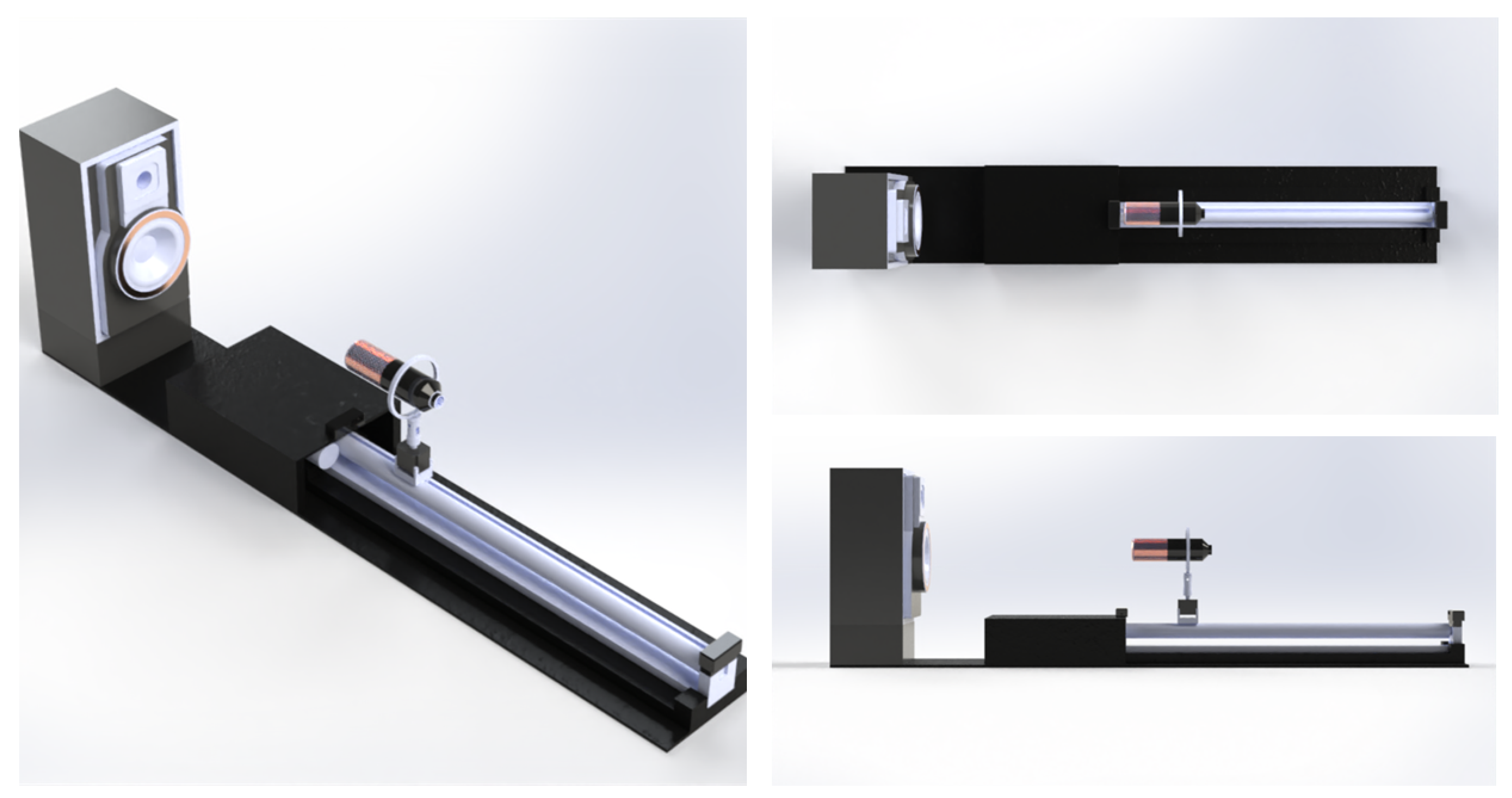
Figure 4.
CAD model of the vent caps and gasket.
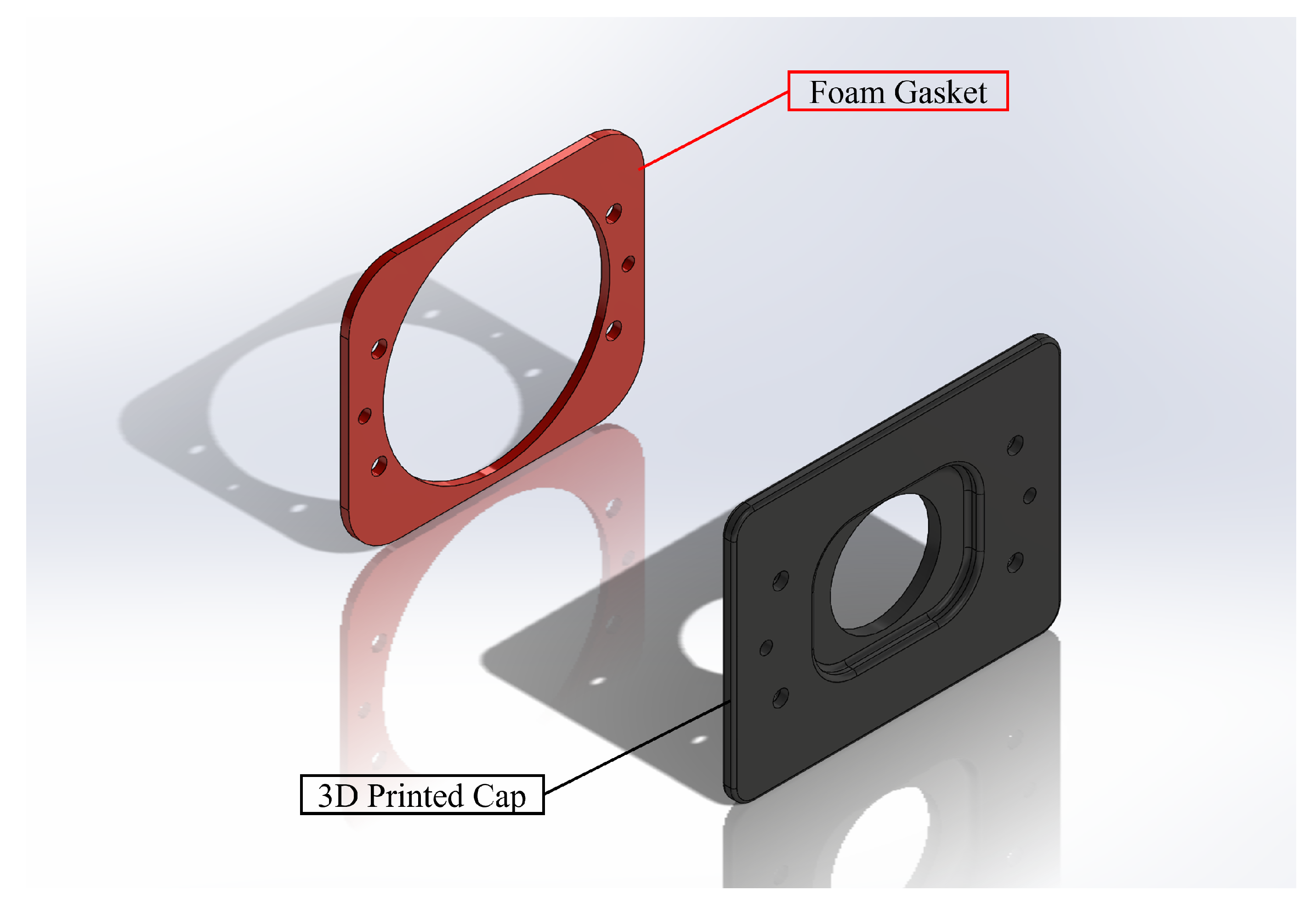
Figure 5.
EAAS hardware setup.
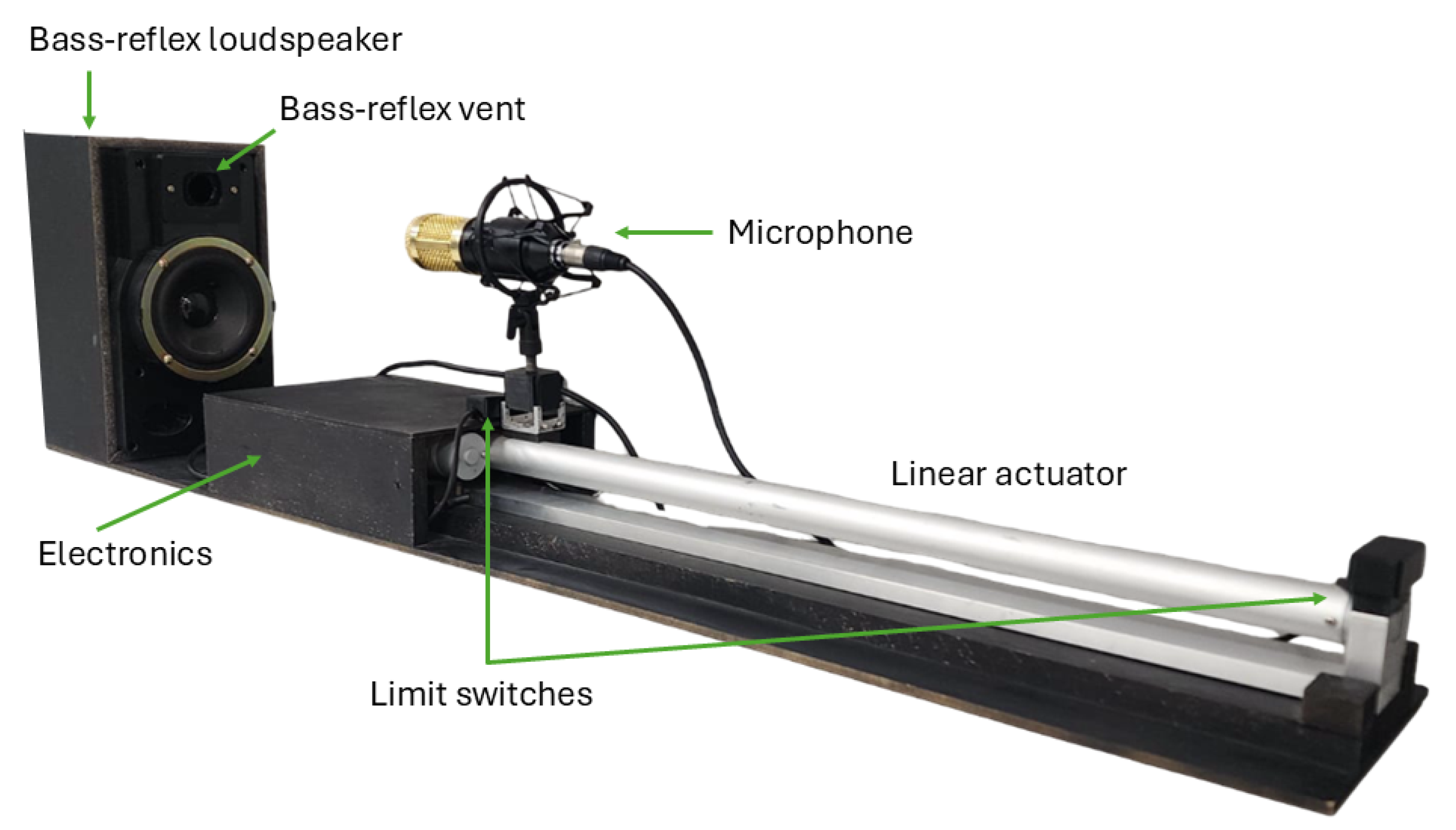
Figure 6.
MATLAB-based EAAS Toolkit graphical user interface.
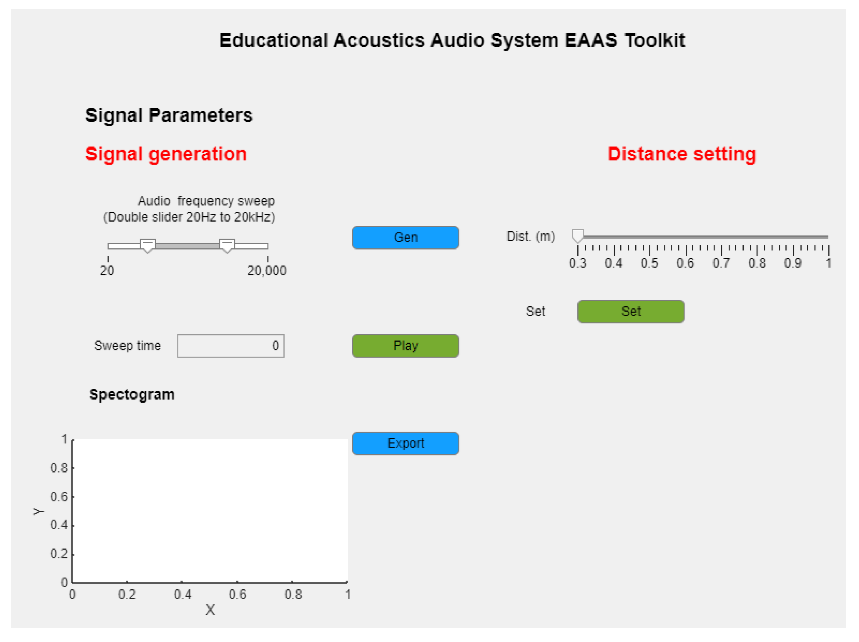
Figure 7.
Microphone positions at three measurement distances. (a) m: near-field position. (b) m: mid-range position. (c) m: far-field position.
Figure 7.
Microphone positions at three measurement distances. (a) m: near-field position. (b) m: mid-range position. (c) m: far-field position.
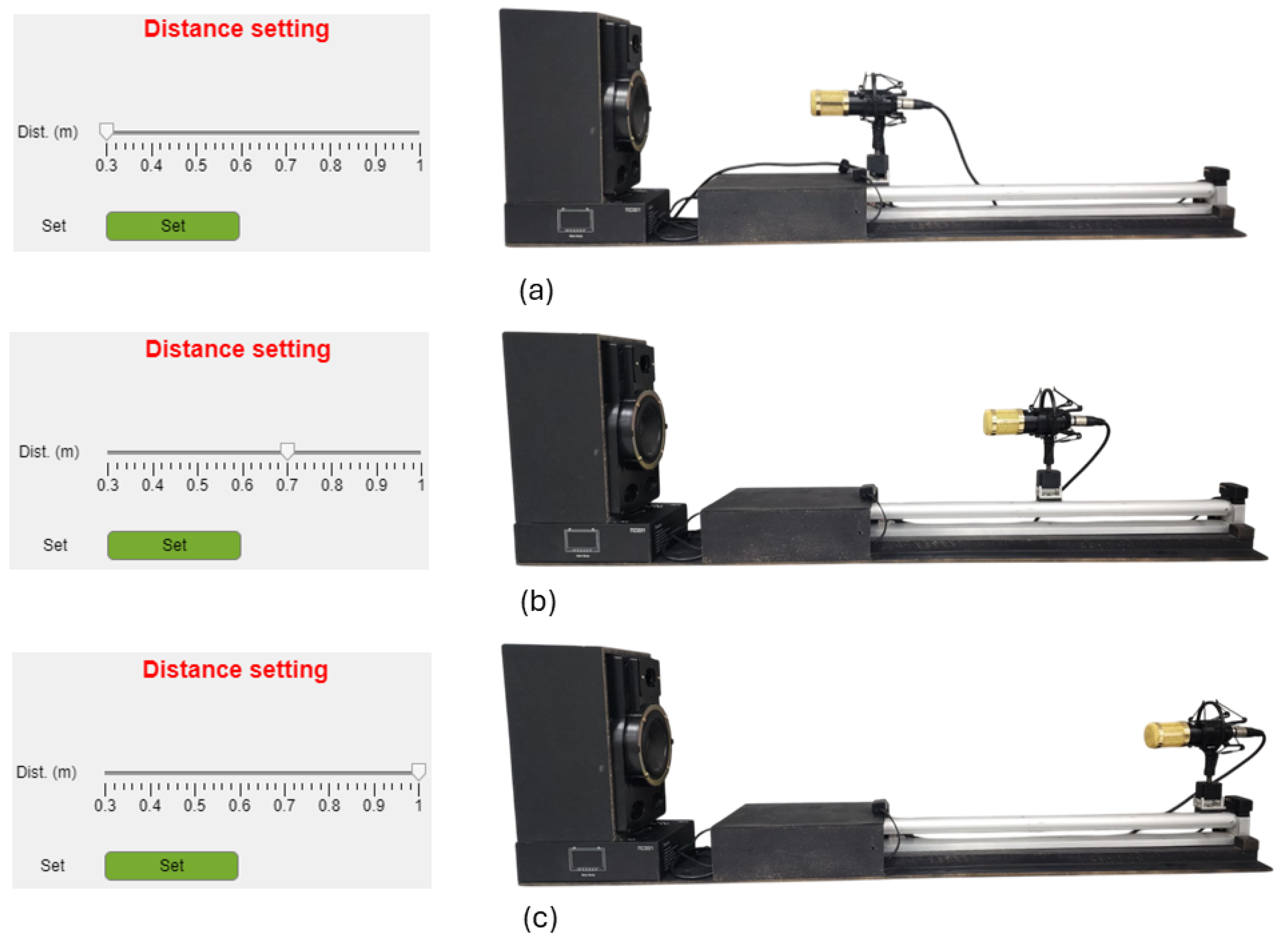
Figure 8.
Spectrogram of the excitation signal.
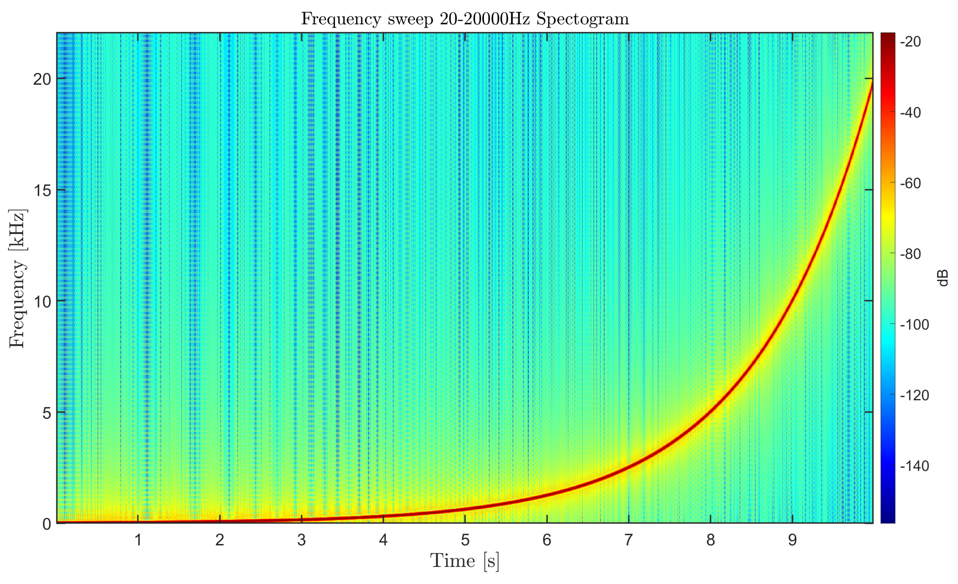
Figure 15.
Full Vent Bass-Reflex Spectogram at 1m.
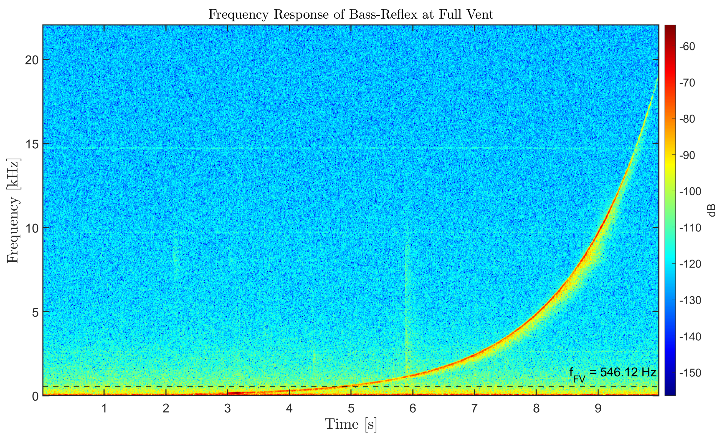
Figure 16.
Half Vent Bass-Reflex Spectogram at 1m.
Disclaimer/Publisher’s Note: The statements, opinions and data contained in all publications are solely those of the individual author(s) and contributor(s) and not of MDPI and/or the editor(s). MDPI and/or the editor(s) disclaim responsibility for any injury to people or property resulting from any ideas, methods, instructions or products referred to in the content. |
© 2025 by the authors. Licensee MDPI, Basel, Switzerland. This article is an open access article distributed under the terms and conditions of the Creative Commons Attribution (CC BY) license (http://creativecommons.org/licenses/by/4.0/).
Copyright: This open access article is published under a Creative Commons CC BY 4.0 license, which permit the free download, distribution, and reuse, provided that the author and preprint are cited in any reuse.


