Submitted:
12 November 2025
Posted:
14 November 2025
You are already at the latest version
Abstract
Traditional CSAMT omnidirectional radiation causes low energy efficiency, while near-field effects and far-field interference limit detection accuracy. To address the issues of energy dispersion, low signal-to-noise ratio, and restricted exploration range in conventional Controlled Source Audio-frequency Magnetotelluric (CSAMT) methods for deep exploration, this paper proposes a tensor CSAMT directional pattern synthesis and adaptive beamforming method based on an L-shaped array artificial field source. An L-shaped source composed of two orthogonal coaxial dipole linear arrays is designed, and Taylor-weighted directional pattern synthesis is employed to reduce sidelobe levels. An adaptive beamforming system is constructed based on the maximum Signal-to-Noise Ratio criterion to achieve dynamic beam steering and energy focusing. Verified via COMSOL simulations and field experiments, this study upgrades the CSAMT artificial source from "omnidirectional radiation" to "directional and controllable" using array antenna technology, providing a high signal-to-noise ratio and efficient electromagnetic detection paradigm for deep resource exploration.
Keywords:
direction diagram synthesis
; tensor CSAMT
; L-shaped array artificial field source
; adaptive beamforming
1. Introduction
Controlled Source Audio-Magnetotellurics (CSAMT) is a frequency-domain artificial source electromagnetic detection technology derived from Audio-Magnetotellurics (AMT) and Magnetotellurics (MT) [1]. In the 1950s, based on an article published by Cagniard, a method for electromagnetic sounding was developed, which calculates apparent resistivity by observing the orthogonal components of natural electric and magnetic fields [2]. Within the audio range (10-1 to 103 Hz), the natural electromagnetic field is relatively weak and there can be considerable human-made interference. In the 1970s, Professor D.W. Strangway and others proposed observing the audio electromagnetic field generated by an artificial source using the AMT measurement method. Since the artificial electromagnetic field allows control over frequency, intensity, and direction, and the observation method is similar to AMT, it is therefore called Controlled Source Audio-Magnetotelluric sounding [3].
Due to the strong absorption of electromagnetic waves by the earth's medium, the detection depth increases as the emission frequency decreases [4], which necessitates increasing the transmission and reception distance (r > 4δ) to satisfy the quasi-plane wave assumption in the far field. Conventional CSAMT employs long-wire sources (1–3 km), equivalent to horizontal electric dipoles, which can be approximated as omnidirectional point sources in the far field (r > 10 km) [5]. Their omnidirectional radiation characteristics lead to significant energy dispersion, with only a small portion of the radiated energy being effectively captured. In addition, long-distance transmission losses and increasing anthropogenic noise interference result in a significant reduction in the signal-to-noise ratio of the received signal, severely limiting detection resolution and data quality [6].
The traditional controlled-source audio-frequency magnetotelluric (CSAMT) method typically relies on increasing transmitter power or reducing the transmission-reception distance to enhance signal amplitude in the far-field region [7]. However, the former is limited by power electronics technology, resulting in bulky equipment and difficulties in field deployment; reducing the transmission-reception distance sacrifices detection depth and introduces significant source field effects [8]. Therefore, it is crucial to develop a new type of source technology that can efficiently utilize radiated energy while maintaining the existing transmitter power. This study focuses on proposing a tensor CSAMT method based on an L-shaped array artificial source and its engineering implementation. The design replaces the two traditionally separated single-dipole sources with two sets of orthogonal coaxial linear dipole arrays forming an L-shaped structure. Field test data fully demonstrate that this array antenna-based artificial source can effectively reduce multipath interference, achieve adaptive directional radiation to specific areas, and significantly improve the signal-to-noise ratio and resolution of exploration data, providing a powerful technical means for deep resource exploration in complex environments. It lays a theoretical foundation for adaptive exploration.
CSAMT is a frequency-domain electromagnetic method that belongs to the artificial source methods. When observations are made in the far-field zone, its data can correctly reflect changes in the geoelectric structure [9]. However, in other areas, due to the influence of artificial sources, non-plane wave effects related to the transmission frequency are generated—in other words, influenced by the transition zone and near zone—resulting in significant distortions in the apparent resistivity curves of the Cagniard method, manifested as a 45° rise at low frequencies on the log-log scale [10]. This is known as the near-field effect. In practical exploration, MT two-dimensional or three-dimensional inversion software can only invert far-field data. However, when measuring in the far-field zone, the signal-to-noise ratio is often not high and is easily disturbed, while shortening the transmitter-receiver distance is affected by near-field effects. This significantly limits the penetration depth of the CSAMT method [11]. Currently, most scholars focus on solving near-field effects and increasing transmitter power, while there is relatively little research on improving the energy utilization of artificial sources. Based on long-offset transient electromagnetic methods, Xue Guoqiang et al. proposed the short-offset transient electromagnetic method. By exciting electromagnetic field signals using grounded line sources and observing the response in the near-source zone along the equator, with offset distances typically 0.5–1.5 times the exploration depth, this method can achieve deep exploration with relatively short offsets [12].
The CSAMT method can use either magnetic field sources or electric field sources as artificial sources. Due to differences in implementation, to achieve the exploration effect of an electric field source, a magnetic field source requires more than 10 times the supply current [13]; therefore, in practice, electric field sources are mainly used. Tensor CSAMT employs two grounded horizontal electric dipole antennas in mutually perpendicular directions, allowing the establishment of a three-dimensional current field underground. Since the grounded horizontal electric dipole antennas in these two directions are independent dipoles with individually varying electromagnetic field components, they can measure a total of 10 components [14]. Tensor CSAMT typically uses two mutually perpendicular sources to establish a three-dimensional current field underground and measure the 10 components of the electromagnetic field. The electromagnetic field components generated by the horizontal dipole are , while those in the perpendicular direction are . All 10 components need to be measured to determine the impedance tensor. Common tensor CSAMT construction instruments include two types: L-shaped sources and cross-shaped sources.
The leftmost type in Figure 1 is the tensor CSAMT cross-shaped field source transmitter, with its core consisting of two sets of horizontal electric dipoles arranged perpendicularly [15]. In operation, the transmitter alternately supplies power to the two electrode pairs (A-B and C-D), thereby generating underground current fields in the x and y directions, respectively. This time-sharing excitation method allows the receiver to independently observe the electromagnetic field responses in the two orthogonal directions. The middle type in Figure 1 is the tensor L-shaped field source transmitter, also composed of two mutually perpendicular horizontal electric dipoles [16]. At a certain point in the far-field region, the electromagnetic field intensities produced by horizontal electric dipole 1 are 、、、, and at the same point, those produced by horizontal electric dipole 2 are 、、、. At that point, the electromagnetic field intensity of the L-shaped field source follows the principle of vector superposition, meaning that the fields from multiple dipole sources can be combined according to vector addition. Therefore, the electromagnetic field at a given point generated by these dipole sources is equal to the vector sum of the fields produced by each dipole at that point.
The rightmost part of Figure 1 shows a schematic diagram of a rotating dipole device, which is different from the two transmission devices above. This device consists of three pairs of dipole transmitters, each made up of three grounded electrodes, A, B, and C. In other words, the three electrodes are respectively connected to the outputs of the tensor transmitter. Under the control of the pulse width modulation controller, the device simultaneously sends the same specified amplitude, frequency, and adjustable polarity currents ,and underground. These three currents combine underground to form the current vector I at the specified frequency. Changing the polarity and amplitude of any of these three currents, according to the vector synthesis principle, will also change the amplitude and polarity of I. Therefore, by selecting the currents , and , electromagnetic field signals in any polarization direction can be obtained.
The antenna system is the core device for transmitting and receiving radio waves, responsible for converting guided waves into electromagnetic waves and vice versa. Basic antennas can handle conventional tasks, but modern radio systems demand higher performance, such as low sidelobe anti-interference [17], specific beam coverage, and spatial scanning [18]. To address these needs, array antenna technology arranges multiple identical antenna elements in a regular linear or planar configuration, applies excitation to them, and leverages electromagnetic wave interference to achieve enhanced directivity or beam control [19]. Developed since the mid-20th century, this technology has been applied in radar, satellite communications, resource exploration, and environmental monitoring [20], and has spurred the development of pattern synthesis technology to optimize performance.
The radiation pattern of an array antenna can be flexibly controlled by adjusting the number of elements, layout, excitation amplitude, and phase [21]. For different application scenarios, such as low sidelobe anti-interference, null suppression, or flat-top beam coverage, the pattern shape needs to be customized [22]. The main methods for pattern synthesis include deterministic synthesis (achieving precise correlation through mathematical functions [23]) and stochastic synthesis, which relies on random or global optimization algorithms [24].
1) Deterministic Synthesis Methods: These include two methods for uniform array needle beams: the Dolph-Chebyshev synthesis method and the Taylor synthesis method [25], as well as two methods for shaped pattern synthesis: the Woodward-Lawson and Elliott-Stern synthesis methods [26].In array antenna pattern synthesis, Dolph initially used Chebyshev polynomials to optimize the performance of side-lobe arrays [27], controlling the excitation amplitude through polynomial coefficients to minimize the main lobe width at a fixed side-lobe level. However, when the number of array elements increases, this method reveals some drawbacks, such as all-equal side-lobes wasting radiated power and uneven edge current distribution. Taylor addressed these issues by utilizing the side-lobe attenuation characteristics of the sampling function (Sa function), combining the Sa function with the ideal spatial factor of a line source, and proposing the Taylor synthesis method [28], which decreases the side-lobe level starting from the nth side-lobe while keeping equal side-lobes in the main beam region. This method has become mainstream for low side-lobe synthesis, and deterministic synthesis methods are characterized by low computational load and high speed.
2) Uncertainty Synthesis Algorithms: Global optimization algorithms or stochastic optimization algorithms are a class of algorithms for solving non-convex optimization problems to search for the global optimum [29]. Common algorithms include genetic algorithms, simulated annealing, particle swarm optimization, cross-entropy algorithms, differential evolution algorithms, and so on [30]. These methods are mainly applied to non-convex optimization problems in array antenna pattern synthesis, such as array sparsity, and can achieve good results [31]. However, these global optimization algorithms are computationally intensive, and the computation increases rapidly as the number of unknowns grows [32].With social progress, human-made interference in the environment has become increasingly severe, and electronic noise poses a significant threat to CSAMT data reception [33]. Artificial source antennas act as spatial filters in exploration [34], serving as the first line of defense against interference in CSAMT [35]. Antenna anti-interference technologies mainly include low-sidelobe/ultra-low-sidelobe designs, sidelobe masking, adaptive sidelobe cancellation, adaptive array systems, beam control, antenna coverage, and scanning control, among others [36]. Conventional single-dipole antennas and non-adaptive array antennas have fixed beam directions, making it impossible to automatically track the reception point while suppressing interference, which makes it difficult to meet the exploration requirements in complex electromagnetic environments [37].
The fundamental difference between adaptive beamforming and non-adaptive beamforming (i.e., pattern synthesis) lies in the method for determining weights: the former calculates the element weights dynamically based on real-time received signals, while the latter sets fixed weights according to a predesigned target pattern. The pattern of adaptive beamforming can change adaptively with interference signals and noise environments, thereby significantly improving resolution and interference suppression capabilities. As an emerging approach, adaptive array antenna technology achieves real-time beam control through algorithms, with the core objective of autonomously aligning the direction of receiving units while maintaining low sidelobe characteristics of the main beam, maximizing the amplitude of received electric field signals, and effectively suppressing or reducing interference intensity.
Based on the fixedness of the weight vector, beamformers can be divided into adaptive and conventional types [40]. The conventional type uses a fixed weight vector, which is simple to implement but limited by the uncertainty of the received signal, resulting in restricted estimation performance [41]. Adaptive beamforming technology dynamically optimizes the weight vector using received data and specific design criteria such as minimum mean square error, minimum variance, constant modulus, or maximum signal-to-interference-plus-noise ratio (SINR) criteria, enhancing interference suppression and improving resolution [42]. This paper focuses on the adaptive beamforming method based on the maximum SINR criterion, conducting an in-depth study of adaptive beamforming techniques for L-shaped array field sources, with particular emphasis on exploring the algorithm's potential in suppressing side interference and dynamically optimizing beam direction. Its ultimate value lies in providing a novel intelligent field source solution for high-precision tensor CSAMT exploration.
2. Theoretical Foundation
2.1. CSAMT Basic Equations
In electromagnetic detection, the skin depth reflects the depth of electromagnetic exploration. Chen Weiying and others further proposed the concept of effective skin depth, extending the definition to the entire field domain, that is, the depth at which the amplitude of the electromagnetic field from an artificial source decays to 1/e of the surface amplitude [44]. Studies show that the effective skin depth of different electromagnetic field components is correlated with the medium's conductivity, the transmission frequency, and the transmitter-receiver distance. Chen Mingsheng and others pointed out that the actual depth of artificial source electromagnetic detection is controlled not only by the frequency and resistivity but also by the transmitter-receiver distance and ground electrical section parameters. The electromagnetic field of CSAMT is divided into near, transition, and far zones based on the distance from the source; only in the far zone can it be approximated as a plane wave field, allowing the detection depth to be directly estimated using the skin depth [43]. The near-field is independent of frequency and loses depth measurement capability, so it is necessary to increase the transmitter-receiver distance to meet far-zone conditions, thereby enhancing detection depth and stratigraphic resolution. In the far zone, when electromagnetic waves at a certain frequency propagate within a half-space, and the ratio of the electromagnetic wave amplitude at a point on the surface to the amplitude at a certain depth beneath that point is e, that depth is defined as the skin depth of the electromagnetic wave at that frequency, with the expression::
In the formula, is the skin depth, is the resistivity, represents the frequency of the electromagnetic wave, and represents the wavelength of the electromagnetic wave.
Cagniard apparent resistivity is the core method for calculating apparent resistivity using the CSAMT method. Its formula is based on the assumption of a uniform half-space, and it is mainly applicable in the far-field region, where electromagnetic waves enter the subsurface in a quasi-plane wave form, allowing the apparent resistivity to objectively reflect the vertical changes of the subsurface electrical section. In the near-field or transition zones, however, the calculated results can be severely distorted due to non-plane wave effects and cannot represent the true subsurface electrical structure. In actual field surveys, the formula needs to be corrected. At the measurement points, the corresponding frequency components of the electric field and the orthogonal horizontal magnetic field component are measured successively, and the Cagniard apparent resistivity and impedance phase are calculated using the formula:
In the formula, is the magnetic permeability; ; is the frequency; is the phase of the magnetic field component ; is the phase of the electric field component . By sweeping the frequency from high to low, the variation characteristics of the Kani resistivity with frequency can be obtained, thus enabling frequency-domain sounding observations.
Tensor CSAMT uses two overlapping or separate artificial field sources to measure 10 electromagnetic field components(和). Tensor CSAMT can provide more information about subsurface targets and is generally used to investigate complex or anisotropic geological bodies.
Currently, tensor CSAMT measurements are mainly implemented through separated (left of Figure 2) and overlapping field sources (right of Figure 2). Both methods use two independent single electric dipole sources to inject alternating currents into the ground, thereby exciting electromagnetic fields. The vector superposition and interference effects of electromagnetic waves in the far-field region are then used to obtain more complete tensor electromagnetic field data. The core difference lies in the spatial arrangement: in the separated layout, the distance between field sources is relatively large, causing significant interference of the electromagnetic waves along the propagation path; in the overlapping layout, the field sources are positioned almost identically, with the electromagnetic waves being co-located in origin, resulting in relatively minimal interference.
Whether using scalar, vector, or tensor measurements, the radiation pattern obtained from theoretical calculations and simulations shows that within the 360° angular range, each component of the electromagnetic field has certain weak areas, referred to as 'null zones.' Therefore, to ensure data quality, the measurement area is strictly limited, and it becomes difficult to perform measurements once outside this area.
2.2. Array Antenna Theory
Array antennas can be classified into two types: non-adaptive and adaptive [46]. Non-adaptive antennas use preset fixed weights and cannot respond to changes in the external environment [47], which limits their range of applications. Adaptive antennas, on the other hand, can adjust their weights in real time. Through the adaptive beamforming (AB) process [48], they enhance the output in the direction of the desired signal while suppressing interference. Thanks to the interference and superposition effects of electromagnetic waves, array antennas (such as combinations of multiple radiators) achieve superior radiation characteristics compared to a single antenna through spatial energy reorganization. When analyzing the radiation problem of a specific current source, the distribution of the current source is usually specified first, and then the radiation field generated by that specific current source is calculated. For a given time-harmonic current source J, the vector magnetic potential A is usually introduced to obtain its radiated electromagnetic field. It can be derived that:
Array antennas achieve flexible control of electromagnetic wave radiation characteristics through the cooperative operation of multiple elements. The core principle lies in utilizing the interference effect of electromagnetic waves in space. By precisely controlling the excitation amplitude and phase of each element, the radiated electromagnetic field can coherently add or cancel in specific regions, thereby forming directional beams or specific radiation patterns49. This interference phenomenon gives array antennas design freedoms far beyond those of a single antenna, enabling them to meet high-level requirements for beam shape, directionality, and anti-interference capability in complex application scenarios50. In a uniform medium, the radiated electromagnetic field produced by multiple correlated source currents follows the principle of vector superposition, and its total field can be expressed as:
Here, represents the vector magnetic potential of the current source; represents the relative magnetic permeability of the medium; represents the dielectric constant of the medium. According to the wave equation:
Here, represents the linear current density of a linear radiating source, which also applies to a planar radiating source. As shown in Figure 3, the linear current density is along the y-axis.
If the length of a linear current source is, and is the distance between the linear current source and an observation point P in space, then the vector magnetic potential at the observation point in space is given by equation (7). If a linear radiating source is equivalent to small current elements, then the vector magnetic potential at any point in space generated by each element, when superimposed, gives the total radiated field according to equation (8). Therefore, whether it is a linear or planar current source, the magnetic vector potential of the total field follows the principle of superposition and can be equivalently represented by a discrete array of sources.
A linear array consists of N isotropic antenna elements arranged coaxially along the x-axis. Let the nth element be at a distance from the origin, as shown in Figure 4.
and are the amplitude ratio and phase difference of the nth element compared to the first element. The complex current of the nth array element is expressed as:
According to the principles of electromagnetic wave interference and superposition, assuming point P is located infinitely far from the array in space, the radiation field of the linear array at this point is:
Based on the principle of electromagnetic wave interference and superposition, the pattern map product theorem is established, and , and are used to represent the pattern map, array factor and unit pattern function of the antenna array:
According to Equation (10), the pattern diagram function of an array antenna is determined by the product of the element pattern and the array factor, which is the pattern product theorem. The theorem is established under the influence of neglect or the coupling of the alignment elements. The array factor characterizes the influence of the geometric layout, spacing and excitation amplitude phase distribution of the array on the radiation characteristics, which can be regarded as the direction function of the point source array. Therefore, by optimizing the array factor (Equation 10), the overall directional performance of the array can be effectively controlled under the premise of fixing the element pattern. When the array elements are equally excited and the phase center is at the origin, the normalized array factor can be simplified to Equation (12). For a rectangular plane matrix arranged in a rectangular grid, if the excitation amplitude of each element can be separated (), the result of multiplying the patterns of the two orthogonal linear arrays is the pattern of the plane array.
As shown in Figure 5, in the xy plane, there is a rectangular grid planar array with elements, with row spacing and column spacing .
The coordinate position of the mnth unit is:
The position vector is , and the excitation current of the first element is , and the radiation field in the far field is represented as follows:
Path difference is:
Then the far-field radiation of the mn-th element is:
The far-field radiation of the entire planar array is:
According to the theorem of the product of directional diagrams, the array factor in the formula is:
If the planar array is distributed by column as and by row as , then
and are the amplitude distributions of linear arrays arranged along the x and y directions; and are the uniform phase increments of the linear arrays arranged along the x and y directions. Substituting equation (19) into the array factor formula gives:
For a uniform planar array, , we can obtain:
When , the maximum value of occurs, and when and are the maximum beampointing, then . In the same way, when , the maximum value of occurs, and when and are the maximum beam direction, then .
3. Simulation Study of L-Shaped Array Adaptive Directional Pattern
3.1. Traditional Separated Tensor CSAMT Simulation
The traditional separation tensor CSAMT model based on a single electric dipole antenna artificial field source is shown in Figure 6. Its half-space parameters and the single electric dipole antenna artificial field source parameters are the same as those of the previously mentioned CSAMT model based on a linear array artificial field source. The model consists of a sphere with a radius of 10 km, where the upper half-space is an air domain (, and ), and the lower half-space is a soil domain (, and ).
In the model, two single electric dipole antenna artificial field sources, each with an arm length of 1 km and an arm radius of 0.05 m, are placed on the surface of the ground. They are located at two corners of an isosceles right triangle with a hypotenuse of 8 km and positioned perpendicular to each other at 90º. Each single electric dipole antenna artificial field source applies an alternating current of 50 kW.
Figure 7, Figure 8 and Figure 9 illustrate the electromagnetic field interference phenomenon of two single electric dipole antennas in traditional separated tensor CSAMT under in-phase excitation. When the antennas are excited in-phase, the radiated energy flow splits into five beams due to interference. Measurement lines usually start from the cross point midway between the two antennas and extend outward along the central beam. This cross point is an ideal starting location for tensor measurements because the electric and magnetic field components are balanced, the energy flux density is high, and the signal-to-noise ratio (SNR) is even. As the distance increases, the energy gradually attenuates, limiting the measurement area.
Figure 7 shows the amplitude and direction of the electric field. The direction of the electric field is always parallel to the orientation of a single dipole, forming a linearly polarized electromagnetic wave. The electromagnetic wave propagates in a 'beam' pattern, which results from the interference and superposition of electromagnetic waves, that is, the electromagnetic waves from the two antennas interfere with each other, redistributing the energy. Where the electric field is strong, the magnetic field is weak, and vice versa, in accordance with the law of conservation of energy. This phenomenon requires a certain distance between the two antennas; if the antennas are co-located, the differences between the waves do not change with the observation angle, and directional selective interference cannot be produced.
Figure 8 shows the magnetic field amplitude and direction. According to electromagnetic wave propagation theory, the magnetic field and electric field induce each other and are orthogonal. In the figure, it is clearly seen that the direction of magnetic field oscillation is always perpendicular to the orientation of a single electric dipole. Figure 9 shows the direction of the Poynting vector, which represents the direction of energy flow; both the electric and magnetic field directions are perpendicular to it.
3.2. L-Shaped Array Field Source Adaptive Pattern Synthesis Simulation
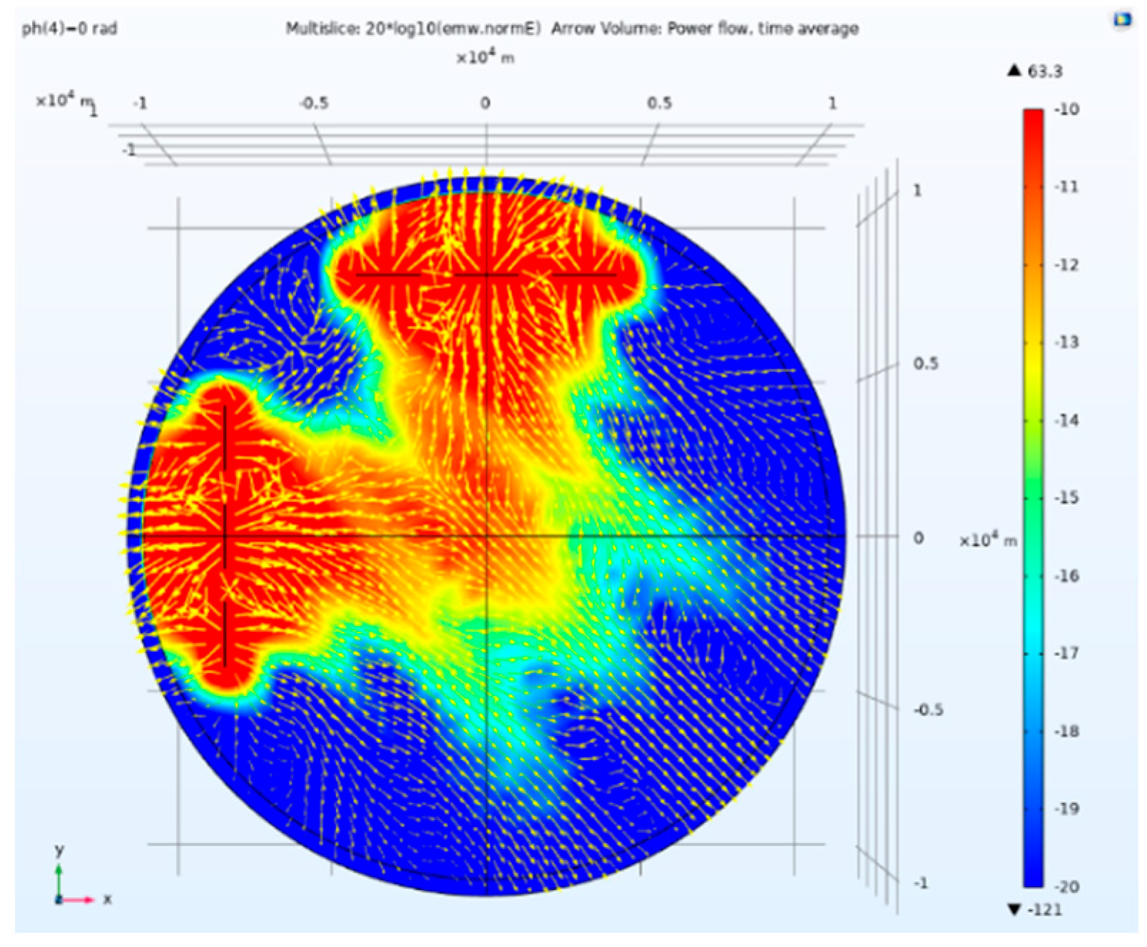
The tensor CSAMT model based on the L-shaped array artificial source is shown in Figure 10. By replacing the single electric dipole sources in the traditional separated configuration with two sets of coaxial linear arrays of oscillators, comprehensive control of the radiation pattern and adaptive beam steering is achieved. The electric field amplitude and direction when the two sets of perpendicular separated coaxial linear arrays of the L-shaped array artificial source are excited with equal amplitude are shown in Figure 11.
Figure 12.
Side view of magnetic field amplitude and direction of tensor CSAMT based on L-type array artificial field source under equal scale excitation.
Figure 12.
Side view of magnetic field amplitude and direction of tensor CSAMT based on L-type array artificial field source under equal scale excitation.
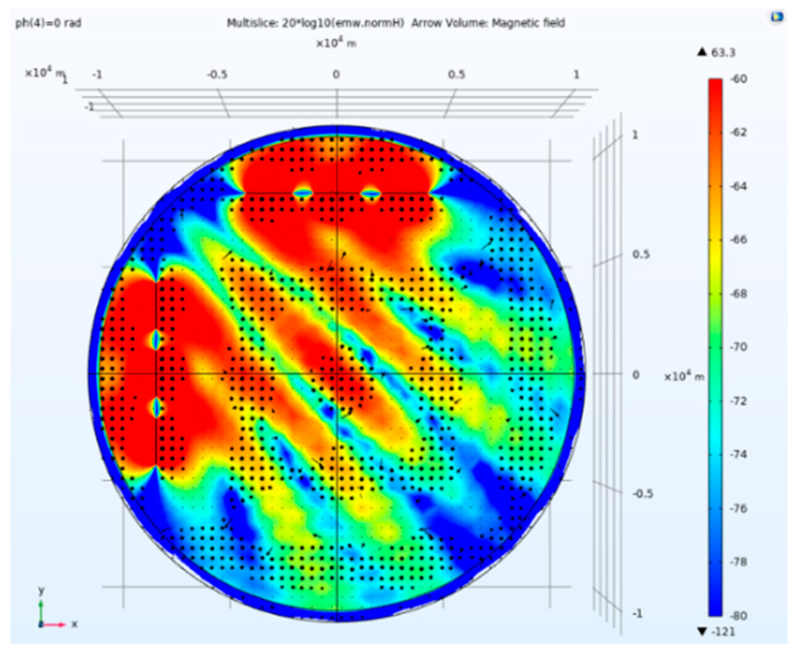
When a total power of 50kW with equal amplitude excitation is applied to the 3×1 coaxial dipole linear arrays on both sides of the L-shaped array, meaning that each of the three array elements is supplied with 720V AC, the uncombined pattern exhibits high sidelobe levels, causing the main lobe energy to disperse and interfere with the receiving points. The beams of the two arrays interfere and superimpose, resulting in a 45° deflection in the propagation direction of the synthesized beam.
According to the principles of electromagnetic field interference and energy conservation, magnetic field energy is distributed in multiple beams and is complementary to electric field energy: where the magnetic field is strong, the electric field is weak, and vice versa. This distribution allows the energy beams to 'fit together' in space, similar to a mortise-and-tenon structure. Therefore, compared with Figure 11, the energy beams in the two diagrams can 'fit together.' Figure 13 further shows the direction of the Poynting vector, which indicates the direction of energy flow, perpendicular to both the electric and magnetic fields, suggesting that interference between the two coaxial oscillator arrays causes the beam propagation direction to deflect 45°, radiating toward the lower right corner. At this point, the central cross point in the figure has relatively high electric field intensity, with balanced electromagnetic field components in the x and y directions, which is the traditional measurement region. However, since the beam has not undergone adaptive adjustment, the exploration range is limited, and energy at the periphery decays rapidly.
Figure 14 and Figure 15 show the electric field amplitude and direction, magnetic field amplitude and direction, and Poynting vector direction when a total power of 50 kW Taylor weighting is applied to a 3×1 coaxial dipole linear array in an L-shaped artificial field source, with the three array elements respectively receiving AC excitations of 502 V, 1055 V, and 502 V. Compared with equal-amplitude excitation as in Figure 11, Taylor synthesis significantly improves the radiation pattern performance, with the sidelobe levels and number noticeably reduced, effectively decreasing multipath interference at receiving points. Due to energy conservation, the reduction of sidelobes enhances the main lobe energy, creating an optimization effect of “gain at the expense of loss,” thereby significantly improving the signal-to-noise ratio (SNR) of the received signals. Theoretically, completely eliminating sidelobes could achieve an infinite SNR, but this is difficult to achieve in practical exploration. This study demonstrates that pattern synthesis effectively suppresses sidelobes, and from the perspectives of energy utilization and anti-interference capability, the method significantly enhances the exploration accuracy and resolution of tensor CSAMT. Figure 15 also shows that the magnetic field energy is redistributed, with a complementary relationship to the electric field energy, generated through mutual induction.
Figure 16.
Side view of electric field amplitude and Poynting vector direction of separation tensor CSAMT based on L-type array artificial field source under Taylor weighted excitation.
Figure 16.
Side view of electric field amplitude and Poynting vector direction of separation tensor CSAMT based on L-type array artificial field source under Taylor weighted excitation.
In the uniform half-space model shown in Figure 10, the linear arrays of coaxial dipoles on both sides of the L-shaped array use Taylor weighting (502V, 1055V, 502V) with variable phase excitation. By setting the port phases to change arithmetically (element 1 at 0 rad; element 2 varying from -0.69813 rad to -2.0944 rad; element 3's phase difference is twice that of element 2), as shown in Table 1, this rule is used to control the direction of the main lobe.
Figure 17, Figure 18 and Figure 19 show the side view of the electric field amplitude and direction after Taylor weighting is applied to the separated tensor CSAMT based on an L-shaped array artificial field source, with phase differences of 0.69813 rad, 1.3963 rad, and 2.0944 rad applied, respectively. It can be seen that as the phase difference increases, the edges of the beam shift outward, demonstrating that as the phase difference increases, the beam scans from the cross point along the 45° line toward the lower right corner. When performing L-shaped field source tensor CSAMT, as excitations with different phase differences are applied, the beam direction will change accordingly.
Now let's observe the beam scanning from the perspectives of the magnetic field and the Poynting vector. Consistent with the electric field situation, the beam energy also flows diagonally 45° toward the lower right, as shown in Figure 20, Figure 21, Figure 22, Figure 23, Figure 24 and Figure 25. Figure 20 and Figure 21 show the magnetic field distribution after excitation with phase differences of 1.3963 rad and 2.0944 rad. It can be seen that as the phase difference increases, the main beam's magnetic field energy is pushed outward.
The comparison of electric field amplitudes after applying equal-amplitude excitation and Taylor weighting for traditional tensor CSAMT and separated tensor CSAMT based on L-shaped array artificial field sources is shown in Table 2. The electric field values were measured at points where (x, y, z) are (0, 0, 0), (1000, -1000, 0), (4000, -4000, 0), and (6000, -6000, 0).
As can be seen in Figure 26, whether it is a traditional tensor, L-shaped array with uniform amplitude excitation, or Taylor synthesis, the electric field amplitude is highest at the point (0, 0, 0) and gradually decreases outward. Among them, the electric field values of the L-shaped array with uniform amplitude excitation are higher than those of the traditional tensor CSAMT, and the electric field values of the L-shaped array after Taylor synthesis are even higher than those with uniform amplitude excitation. It can be seen that the application effect of array antennas and the Taylor synthesis method is still quite obvious. As shown in Figure 27, when conducting CSAMT adaptive beamforming exploration based on an L-shaped array antenna artificial field source, with the scanning of the beam, a curve is formed at the receiving end where the electric field amplitude varies with the phase difference. At this point, performing CSAMT tensor exploration based on the phase difference corresponding to the maximum electric field amplitude completes the adaptive beamforming process.
The comparison of electric field amplitudes in Table 3 shows that when the phase difference is 0 rad, the beam points to the center (0,0,0), with the maximum electric field amplitude that decays outward; as the phase difference increases from 0.69813 rad to 2.0944 rad, the beam peak shifts outward, visually illustrating the beam scanning process.
4. L-Shaped Array Field Adaptive Directional Pattern Test
4.1. Conventional Triaxial Test
Figure 28 shows the layout of a traditional separated tensor CSAMT field test. Two sets of single electric dipole artificial sources are placed perpendicular to each other and separated. The white area in the figure represents the conventional survey range, because within this area, the x-axis and y-axis components of the electromagnetic field are roughly equal in amplitude. As a result, the calculated tensor impedance and impedance phase are relatively accurate. Beyond this range, the differences in the electromagnetic field components along the two perpendicular directions are significant, bringing considerable errors to data processing. The green points in the figure denote regular survey points, where the amplitudes of the electromagnetic field components along the two perpendicular directions are relatively large. The amplitudes at the yellow and orange points gradually decrease.
Figure 29, Figure 30 and Figure 31 show the vertical electric field amplitudes at the traditional measuring point, comparison measuring point 1, and comparison measuring point 2, respectively. The data indicate that from the traditional measuring point to comparison measuring point 2, the electric field amplitude gradually decreases: although the amplitude at comparison measuring point 1 is lower than at the traditional measuring point, it can still be used for exploration when external interference is minimal; the electric field amplitude error at comparison measuring point 2 is too large, making it inadequate for tensor measurements.
4.2. L-Shaped Array Field Source Adaptive Beam Pattern Test
Figure 32 shows the field test layout of the tensor CSAMT based on L-shaped array artificial sources. Two sets of linear array artificial sources are placed perpendicular to each other and separated, forming an L-shaped array.
Figure 33, Figure 34 and Figure 35 show the amplitude values of the electric field in two vertical directions at the traditional measurement point and comparison measurement points 1 and 2 in the exploration area, after synthesizing the directional diagram of the tensor CSAMT for an L-shaped array artificial field source. Consistent with the case of a tensor CSAMT using a single dipole antenna artificial field source, the electric field amplitude gradually decreases from the traditional measurement point to comparison measurement point 2. However, due to the directional diagram synthesis, the energy is effectively concentrated. The data show that the measurements at comparison measurement point 2 are still usable, whereas the data at comparison measurement point 2 with a single dipole antenna artificial field source have significant errors.
Figure 36 and Figure 37 show the changes in the electric field amplitude in two vertical directions at comparison measurement points 1 and 2 in the exploration area after performing tensor CSAMT adaptive beamforming with an L-shaped array artificial field source. The setup is consistent with the COMSOL simulation model described in previous chapters, where three elements in each vertical linear array are sequentially excited with different phase differences. In this way, the beam is gradually pushed outward along the white area, achieving the goal of scanning across the explorable area. As can be seen from the figures, as the beam is pushed outward, the amplitude gradually increases, reaching a peak at comparison point 2, consistent with the numerical simulation data, realizing large-scale, strong-amplitude detection within the exploration range.
5. Conclusion
To address the problem of low energy utilization in the far-field region of CSAMT, this study proposes a tensor CSAMT pattern synthesis and adaptive beamforming method based on an L-shaped array of artificial source fields, aiming to improve exploration signal-to-noise ratio and resolution. Through system simulations, numerical modeling, and field tests, the following key conclusions were drawn.:
A tensor CSAMT method based on an L-shaped array artificial field source is proposed, synthesizing a controllable radiation field through two sets of orthogonal coaxial dipole linear arrays. Compared with traditional separated field sources, the L-shaped array has the capability of pattern synthesis and beam scanning, effectively addressing the issues of energy dispersion and limited exploration range in conventional tensor measurements. Based on the maximum amplitude criterion, an adaptive beamforming system is established. By feedback of the electric field data at the receiving end, the phase and amplitude parameters of the transmitting array are adjusted in real time to achieve dynamic beam direction optimization, significantly improving the signal-to-noise ratio in the target area.
A CSAMT adaptive transceiver system based on Beidou RDSS short messages was developed, achieving time synchronization and remote parameter control between the transmitter and receiver. Field tests showed that the system could stably perform beam scanning and energy focusing, verifying the engineering feasibility of the adaptive approach. After combining an L-shaped array with Taylor weighting, the sidelobe level was reduced by about 7 dB, and the main lobe energy was significantly concentrated. With the same transmission power, the effective exploration range was expanded, and the signal-to-noise ratio of the received signal improved, providing technical support for detecting complex geological targets. This study realized the transition of the CSAMT artificial source from 'omnidirectional radiation' to 'directionally controllable' through array antenna technology, offering a new high signal-to-noise, high-efficiency electromagnetic detection paradigm for deep resource exploration.
Although the array antenna artificial field source developed in this project, which can perform pattern synthesis and adaptive beamforming, has achieved good results in simulations and numerical modeling, there are still many issues that need to be addressed, mainly as follows:
(1) Optimization of field source deployment efficiency. The current array antenna-type field source requires far more grounding electrodes than traditional single dipole sources, resulting in a significant increase in field deployment workload. In the future, more efficient deployment solutions and automation technologies need to be studied to balance the contradiction between high-performance exploration and field operation efficiency.;
(2) More comprehensive adaptive acquisition parameters. Currently, adaptive algorithms mainly rely on the criterion of maximizing the electric field amplitude and have not fully utilized magnetic field component information. In the future, the joint optimization acquisition strategy of electric and magnetic field data will be explored to further improve data quality and anti-interference capability through multi-parameter integration.;
(3) Higher device integration. The existing system adopts a separate architecture with GPS timing and Beidou RDSS short message communication. The next step will be to promote the integrated combination of timing and communication functions, utilizing the high-precision timing capabilities of the Beidou system itself, simplifying device configuration, and improving the system's reliability and engineering applicability.
Author Contributions
Conceptualization, H.F.; methodology, H.F.; visualization, Q.S.; project administration, Q.T.; validation, X.S.; Q.S. All authors have read and agreed to the published version of the manuscript.
Funding
This work was supported by the Tianjin Technology Innovation Guidance Special Project (Fund) - Enterprise Science and Technology Commissioner Project. (No. 25YDTPJC00870)
Institutional Review Board Statement
Not applicable.
Informed Consent Statement
Not applicable.
Data Availability Statement
Not applicable.
Acknowledgments
All of the authors thank the referees, editors, and officers of Remote Sensing for their valuable suggestions and help.
Conflicts of Interest
The authors declare no conflicts of interest.
Abbreviations
| CSAMT | Controlled-source audio-frequency magnetotelluric |
| AMT | Audio-Frequency Magnetotellurics |
| MT | Magnetotellurics |
References
- Wang Xianxiang, Di Qingyun, Xu Cheng. Characteristics of Multiple Dipole Sources and Tensor Measurements of CSAMT [J]. Acta Geophysica, 2014, 57(2): 651-661.
- Guo Z, Hu L, Liu C, et al. Application of the CSAMT method to Pb–Zn mineral deposits: A case study in Jianshui, China[J]. Minerals, 2019, 9(12): 726. [CrossRef]
- Boerner D E, Kurtz R D, Jones A G. Orthogonality in CSAMT and MT measurements[J]. Geophysics, 1993, 58(7): 924-934. [CrossRef]
- Wang R, Yin C, Wang M, et al. Laterally constrained inversion for CSAMT data interpretation[J]. Journal of Applied Geophysics, 2015, 121: 63-70. [CrossRef]
- Wang T, Wang K P, Tan H D. Forward modeling and inversion of tensor CSAMT in 3D anisotropic media[J]. Applied Geophysics, 2017, 14: 590-605. [CrossRef]
- He Y, He W, Wong H. A wideband circularly polarized cross-dipole antenna[J]. IEEE Antennas and Wireless Propagation Letters, 2014, 13: 67-70. [CrossRef]
- Li Diquan, Di Qingyun, Wang Guangjie, et al. Application of CSAMT in Fault Detection for the Planning of the Beijing New Area [J]. Advances in Geophysics, 2008, 23(6): 1963-1969.
- Cao H, Wang K, Wang X, et al. Tipper data forward modeling and inversion of three-dimensional tensor CSAMT[J]. Journal of Applied Geophysics, 2021, 193: 104432. [CrossRef]
- Kouadio K L, Xu Y, Liu C, et al. Two-dimensional inversion of CSAMT data and three-dimensional geological mapping for groundwater exploration in Tongkeng Area, Hunan Province, China[J]. Journal of Applied Geophysics, 2020, 183: 104204. [CrossRef]
- He G, Xiao T, Wang Y, et al. 3D CSAMT modelling in anisotropic media using edge-based finite-element method[J]. Exploration Geophysics, 2019, 50(1): 42-56. [CrossRef]
- Xiong Z, Tang X, Li D, et al. Linear source CSAMT response simulation in the 2D anisotropic formation with topography[J]. Journal of Applied Geophysics, 2019, 171: 103861. [CrossRef]
- He Jishan, Xue Guoqiang. Overview of Short-Offset Electromagnetic Detection Technology [J]. Acta Geophysica Sinica, 2018, 61(1): 1-8.
- Routh P S, Oldenburg D W. Inversion of controlled source audio-frequency magnetotellurics data for a horizontally layered earth[J]. Geophysics, 1999, 64(6): 1689-1697. [CrossRef]
- Wang K, Tan H. Research on the forward modeling of controlled-source audio-frequency magnetotellurics in three-dimensional axial anisotropic media[J]. Journal of Applied Geophysics, 2017, 146: 27-36. [CrossRef]
- Zhou J, Wang J, Shang Q, et al. Regularized inversion of controlled source audio-frequency magnetotelluric data in horizontally layered transversely isotropic media[J]. Journal of Geophysics and Engineering, 2014, 11(2): 025003. [CrossRef]
- Basokur A T, Rasmussen T M, Kaya C, et al. Comparison of induced polarization and controlled-source audio-magnetotellurics methods for massive chalcopyrite exploration in a volcanic area[J]. Geophysics, 1997, 62(4): 1087-1096. [CrossRef]
- Ferreira J A, Ares F. Pattern synthesis of conformal arrays by the simulated annealing technique[J]. Electronics Letters, 1997, 33(14): 1187-1189.
- Perini J, Idselis M. Note on antenna pattern synthesis using numerical iterative methods[J]. IEEE Transactions on Antennas and Propagation, 1971, 19(2): 284-286. [CrossRef]
- Ismail T H, Abu-Al-Nadi D I, Mismar M J. Phase-only control for antenna pattern synthesis of linear arrays using the Levenberg-Marquardt algorithm[J]. Electromagnetics, 2004, 24(7): 555-564. [CrossRef]
- Ma Y, Yang S, Chen Y, et al. Pattern synthesis of 4-D irregular antenna arrays based on maximum-entropy model[J]. IEEE transactions on antennas and propagation, 2019, 67(5): 3048-3057. [CrossRef]
- Er M H. Array pattern synthesis with a controlled mean-square sidelobe level[J]. IEEE Transactions on signal processing, 1992, 40(4): 977-981. [CrossRef]
- Yang K, Zhao Z, Liu Q H. Fast pencil beam pattern synthesis of large unequally spaced antenna arrays[J]. IEEE Transactions on Antennas and Propagation, 2012, 61(2): 627-634. [CrossRef]
- Sun G, Liu Y, Chen Z, et al. Radiation beam pattern synthesis of concentric circular antenna arrays using hybrid approach based on cuckoo search[J]. IEEE Transactions on Antennas and Propagation, 2018, 66(9): 4563-4576. [CrossRef]
- Li H, Sun S, Li W, et al. Systematic pattern synthesis for single antennas using characteristic mode analysis[J]. IEEE Transactions on Antennas and Propagation, 2020, 68(7): 5199-5208. [CrossRef]
- Bucci O M, Capozzoli A, D'elia G. Power pattern synthesis of reconfigurable conformal arrays with near-field constraints[J]. IEEE Transactions on Antennas and Propagation, 2004, 52(1): 132-141. [CrossRef]
- Basit A, Qureshi I M, Khan W, et al. Beam pattern synthesis for an FDA radar with Hamming window-based nonuniform frequency offset[J]. IEEE Antennas and Wireless Propagation Letters, 2017, 16: 2283-2286. [CrossRef]
- Zhang R, Zhang Y, Sun J, et al. Pattern synthesis of linear antenna array using improved differential evolution algorithm with sps framework[J]. Sensors, 2020, 20(18): 5158. [CrossRef]
- Owoola E O, Xia K, Ogunjo S, et al. Advanced marine predator algorithm for circular antenna array pattern synthesis[J]. Sensors, 2022, 22(15): 5779. [CrossRef]
- Li M, Liu Y, Guo Y J. Shaped power pattern synthesis of a linear dipole array by element rotation and phase optimization using dynamic differential evolution[J]. IEEE Antennas and Wireless Propagation Letters, 2018, 17(4): 697-701. [CrossRef]
- Morabito A F, Di Carlo A, Di Donato L, et al. Extending spectral factorization to array pattern synthesis including sparseness, mutual coupling, and mounting-platform effects[J]. IEEE Transactions on Antennas and Propagation, 2019, 67(7): 4548-4559. [CrossRef]
- Liu Y, Bai J, Da Xu K, et al. Linearly polarized shaped power pattern synthesis with sidelobe and cross-polarization control by using semidefinite relaxation[J]. IEEE Transactions on Antennas and Propagation, 2018, 66(6): 3207-3212. [CrossRef]
- Yoo I, Imani M F, Pulido-Mancera L, et al. Analytic model of a coax-fed planar cavity-backed metasurface antenna for pattern synthesis[J]. IEEE Transactions on Antennas and Propagation, 2019, 67(9): 5853-5866. [CrossRef]
- Vorobyov S A. Principles of minimum variance robust adaptive beamforming design[J]. Signal Processing, 2013, 93(12): 3264-3277. [CrossRef]
- Nilsen C I C, Hafizovic I. Beamspace adaptive beamforming for ultrasound imaging[J]. IEEE Transactions on Ultrasonics, ferroelectrics, and frequency control, 2009, 56(10): 2187-2197. [CrossRef]
- Elnashar A, Elnoubi S M, El-Mikati H A. Further study on robust adaptive beamforming with optimum diagonal loading[J]. IEEE Transactions on Antennas and Propagation, 2006, 54(12): 3647-3658. [CrossRef]
- Chen S, Sun S, Gao Q, et al. Adaptive beamforming in TDD-based mobile communication systems: State of the art and 5G research directions[J]. IEEE Wireless Communications, 2016, 23(6): 81-87. [CrossRef]
- Zhou C, Gu Y, He S, et al. A robust and efficient algorithm for coprime array adaptive beamforming[J]. IEEE Transactions on Vehicular Technology, 2017, 67(2): 1099-1112. [CrossRef]
- Khabbazibasmenj A, Vorobyov S A, Hassanien A. Robust adaptive beamforming based on steering vector estimation with as little as possible prior information[J]. IEEE Transactions on signal processing, 2012, 60(6): 2974-2987. [CrossRef]
- Blomberg A E A, Austeng A, Hansen R E, et al. Improving sonar performance in shallow water using adaptive beamforming[J]. IEEE Journal of Oceanic Engineering, 2013, 38(2): 297-307. [CrossRef]
- Liao B, Guo C, Huang L, et al. Robust adaptive beamforming with precise main beam control[J]. IEEE Transactions on Aerospace and Electronic Systems, 2017, 53(1): 345-356. [CrossRef]
- Gu Y, Leshem A. Robust adaptive beamforming based on interference covariance matrix reconstruction and steering vector estimation[J]. IEEE Transactions on Signal Processing, 2012, 60(7): 3881-3885. [CrossRef]
- Zhang M, Zhang A, Yang Q. Robust adaptive beamforming based on conjugate gradient algorithms[J]. IEEE Transactions on Signal Processing, 2016, 64(22): 6046-6057. [CrossRef]
- Lenc T, Keller P E, Varlet M, et al. Neural tracking of the musical beat is enhanced by low-frequency sounds[J]. Proceedings of the National Academy of Sciences, 2018, 115(32): 8221-8226. [CrossRef]
- Moore B C J, Vinay S N. Enhanced discrimination of low-frequency sounds for subjects with high-frequency dead regions[J]. Brain, 2009, 132(2): 524-536. [CrossRef]
- Pelletier C, Weladji R B, Lazure L, et al. Zoo soundscape: daily variation of low-to-high-frequency sounds[J]. Zoo Biology, 2020, 39(6): 374-381. [CrossRef]
- Poli L, Rocca P, Manica L, et al. Pattern synthesis in time-modulated linear arrays through pulse shifting[J]. IET Microwaves, Antennas & Propagation, 2010, 4(9): 1157-1164. [CrossRef]
- Jiao Yongchang, Yang Ke, Chen Shengbing, et al. Particle Swarm Optimization Algorithm for Array Antenna Pattern Synthesis [J]. Journal of Radio Science, 2006, 21(1): 16-20.
- Alijani M G H, Neshati M H. A new noniterative method for pattern synthesis of unequally spaced linear arrays[J]. International Journal of RF and Microwave Computer-Aided Engineering, 2019, 29(11): e21921. [CrossRef]
- Liu Y, Liu Q H, Nie Z. Reducing the number of elements in multiple-pattern linear arrays by the extended matrix pencil methods[J]. IEEE Transactions on Antennas and Propagation, 2013, 62(2): 652-660. [CrossRef]
- Wang Z, Sun G, Tong J, et al. Pattern synthesis for sparse linear arrays via atomic norm minimization[J]. IEEE Antennas and Wireless Propagation Letters, 2021, 20(12): 2215-2219. [CrossRef]
Figure 1.
Artificial field source type of tensor CSAMT.
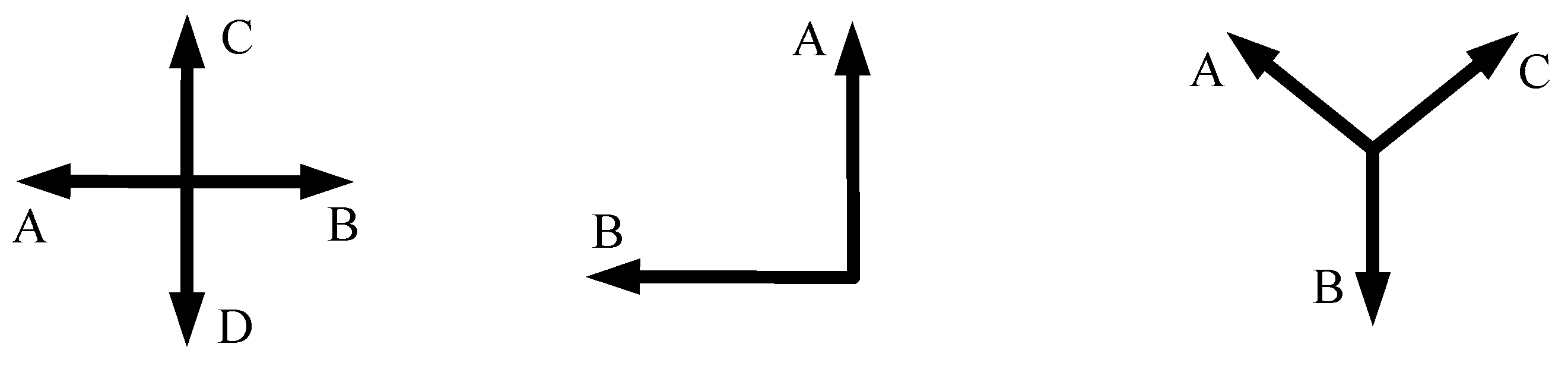
Figure 2.
Tensor CSAMT.
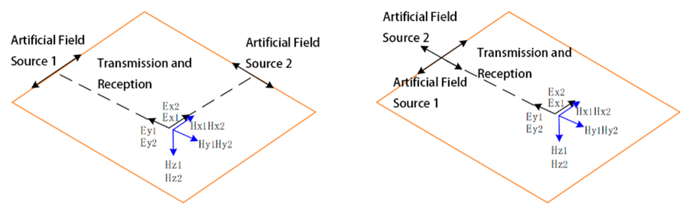
Figure 3.
Linear radiation source.
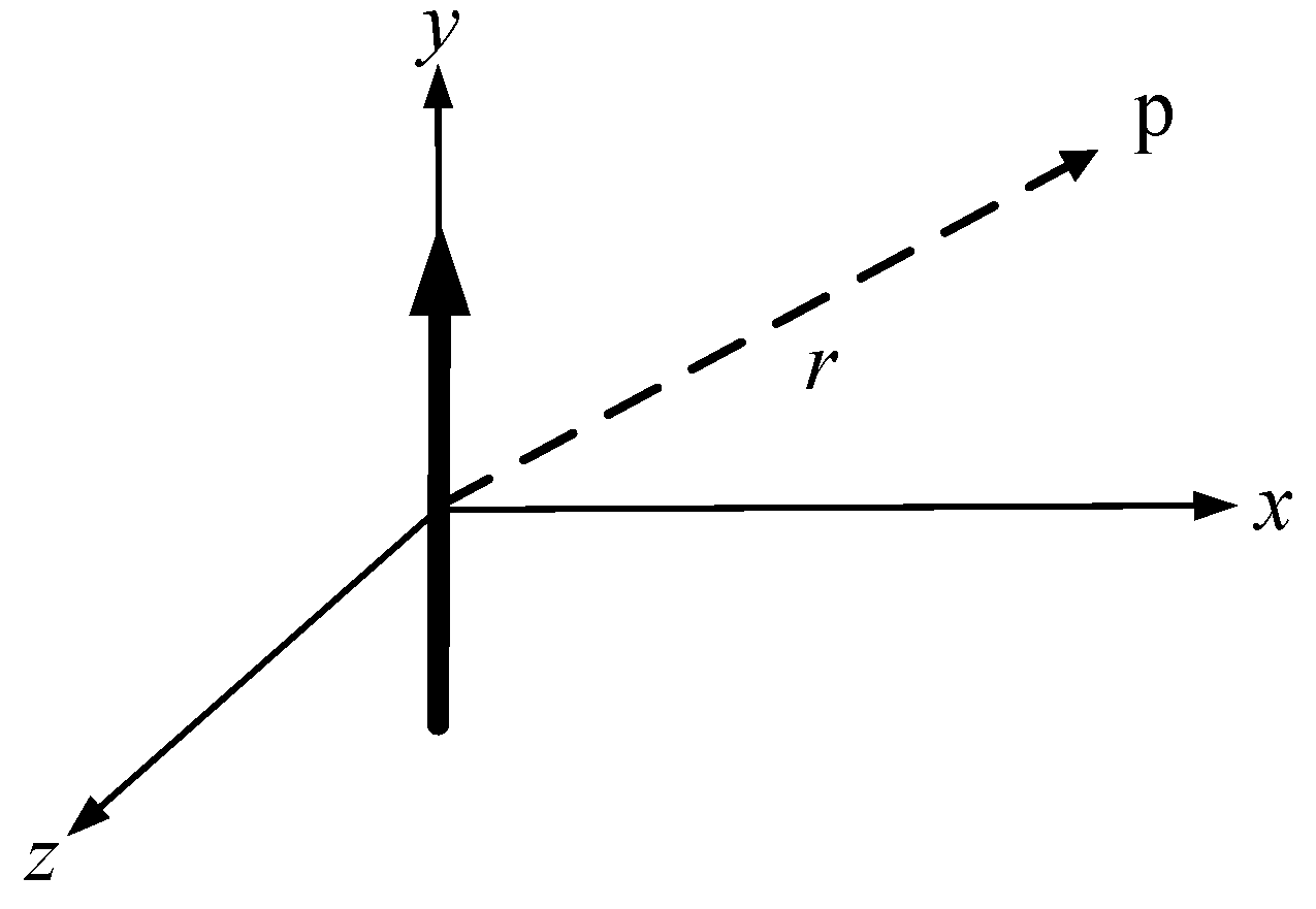
Figure 4.
Uniform linear array.
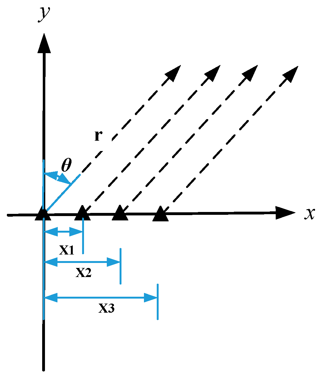
Figure 5.
Uniform planar array.
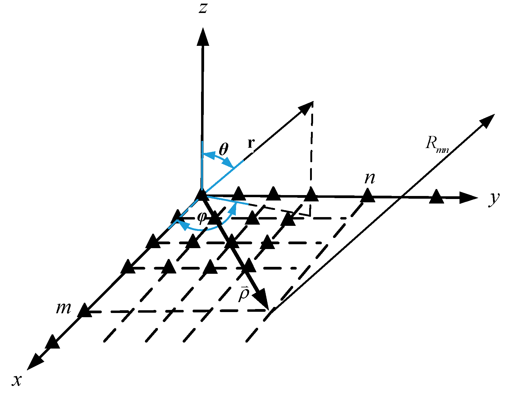
Figure 6.
The traditional separation tensor CSAMT model based on single electric dipole antenna artificial field source.
Figure 6.
The traditional separation tensor CSAMT model based on single electric dipole antenna artificial field source.
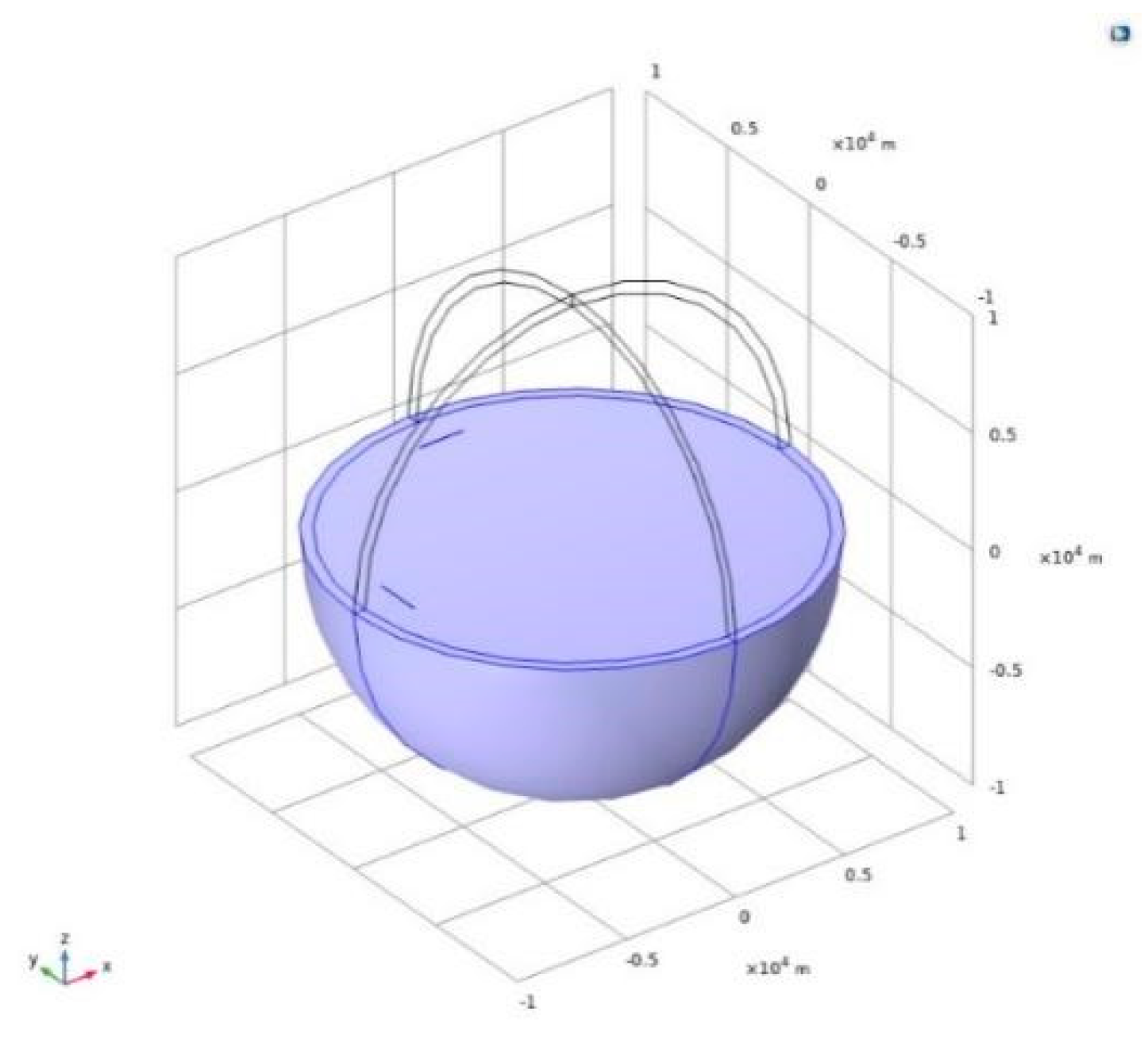
Figure 7.
Side view of electric field amplitude and direction of traditional separation tensor CSAMT.
Figure 7.
Side view of electric field amplitude and direction of traditional separation tensor CSAMT.
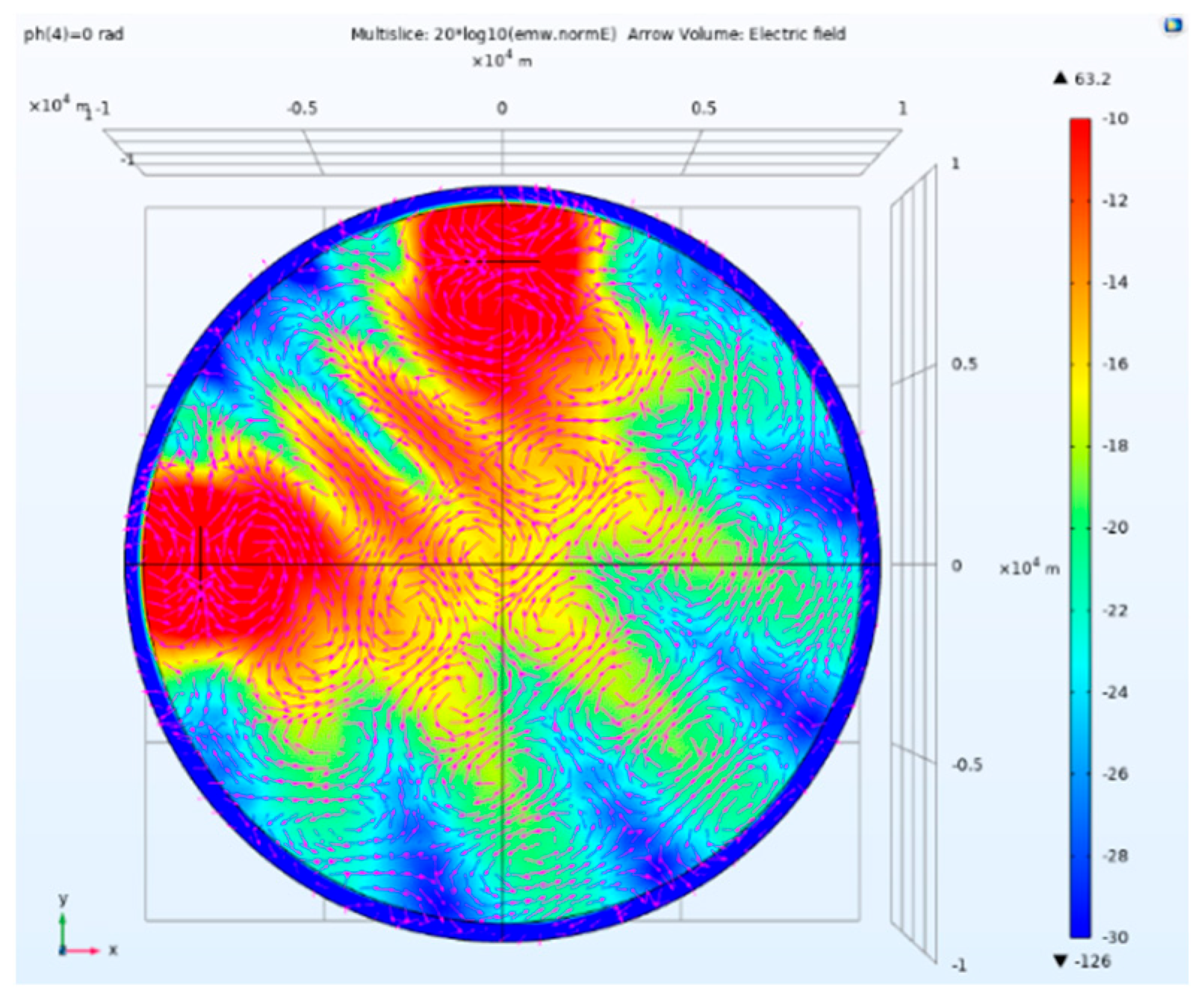
Figure 8.
Side view of magnetic field amplitude and direction of traditional separation tensor CSAMT.
Figure 8.
Side view of magnetic field amplitude and direction of traditional separation tensor CSAMT.
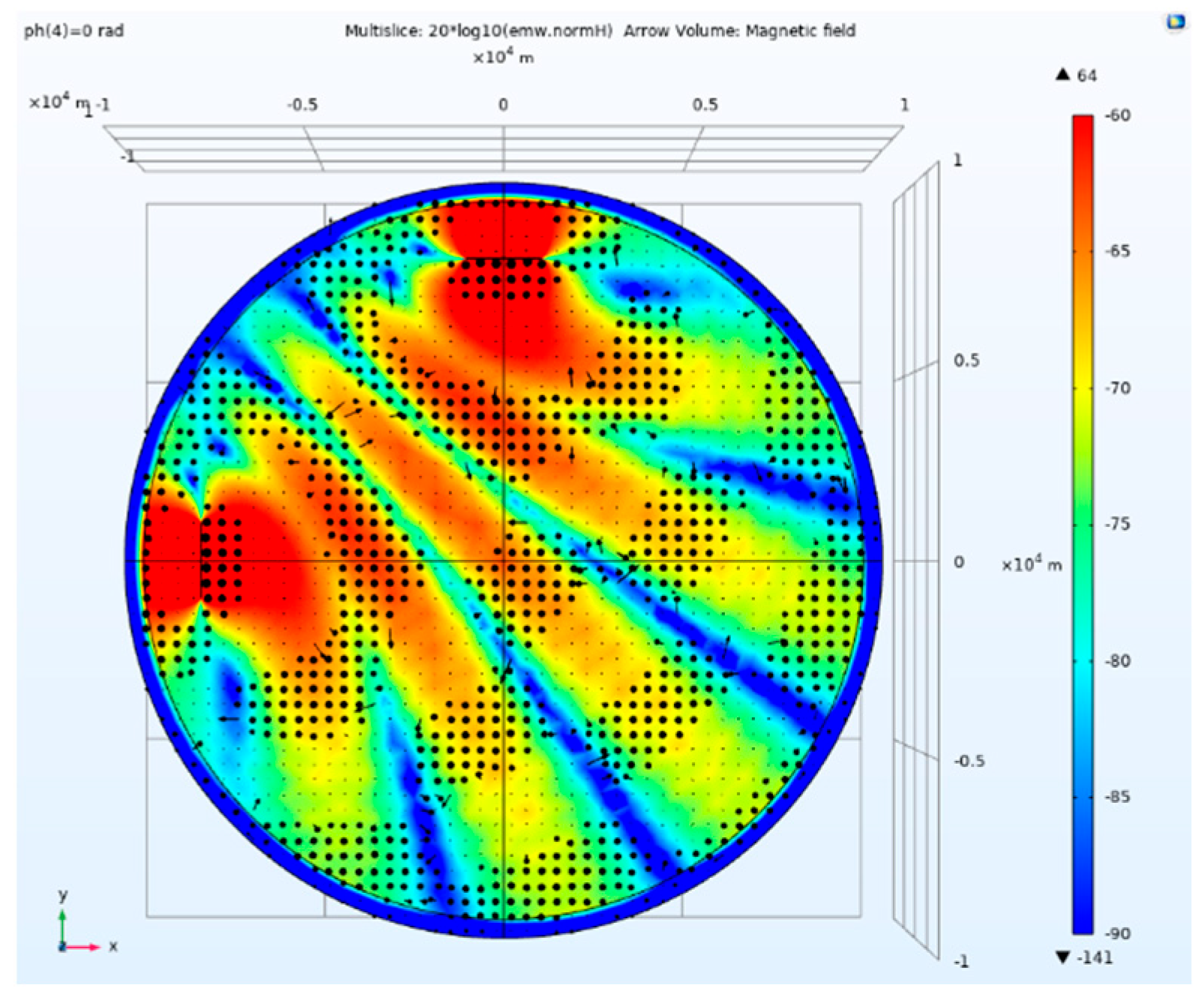
Figure 9.
Side view of electric field amplitude and Poynting vector direction of traditional separation tensor CSAMT.
Figure 9.
Side view of electric field amplitude and Poynting vector direction of traditional separation tensor CSAMT.
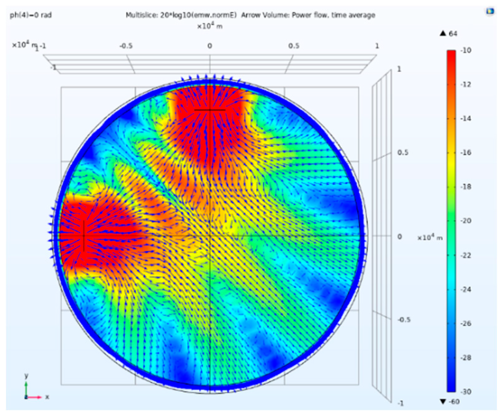
Figure 10.
Separation tensor CSAMT model based on L-type array artificial field source.
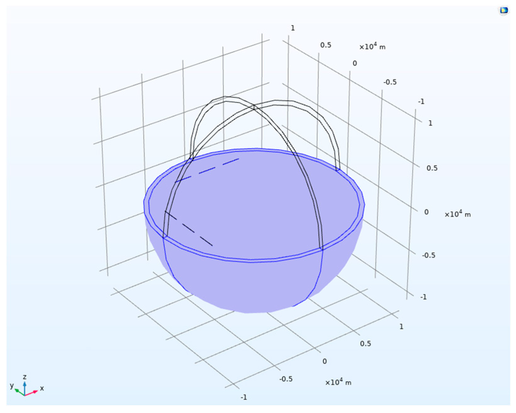
Figure 11.
Side view of electric field amplitude and direction of tensor CSAMT based on L-type array artificial field source under equal scale excitation.
Figure 11.
Side view of electric field amplitude and direction of tensor CSAMT based on L-type array artificial field source under equal scale excitation.
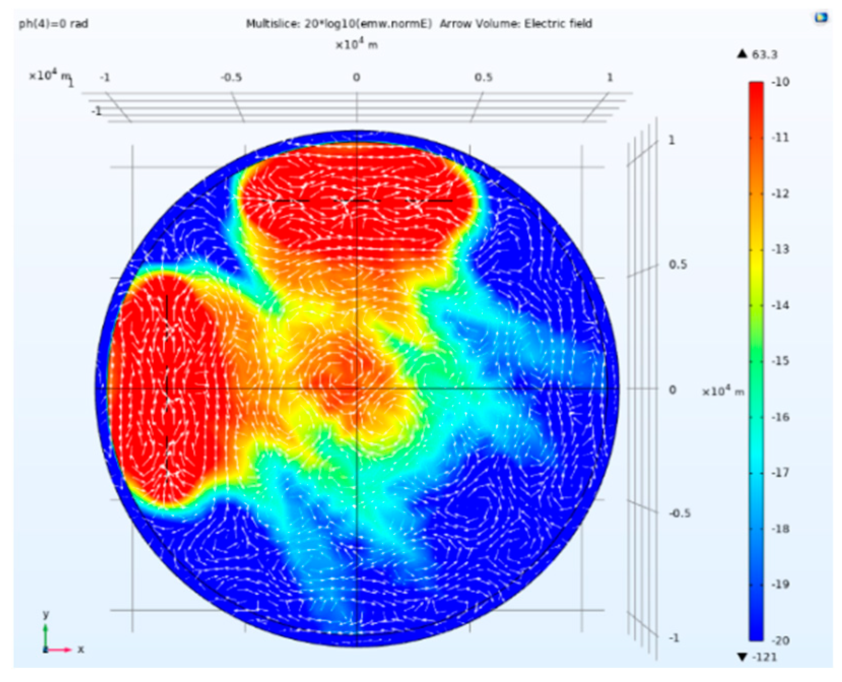
Figure 13.
Side view of electric field amplitude and Poynting vector direction of tensor CSAMT based on L-type array artificial field source under equal scale excitation.
Figure 13.
Side view of electric field amplitude and Poynting vector direction of tensor CSAMT based on L-type array artificial field source under equal scale excitation.
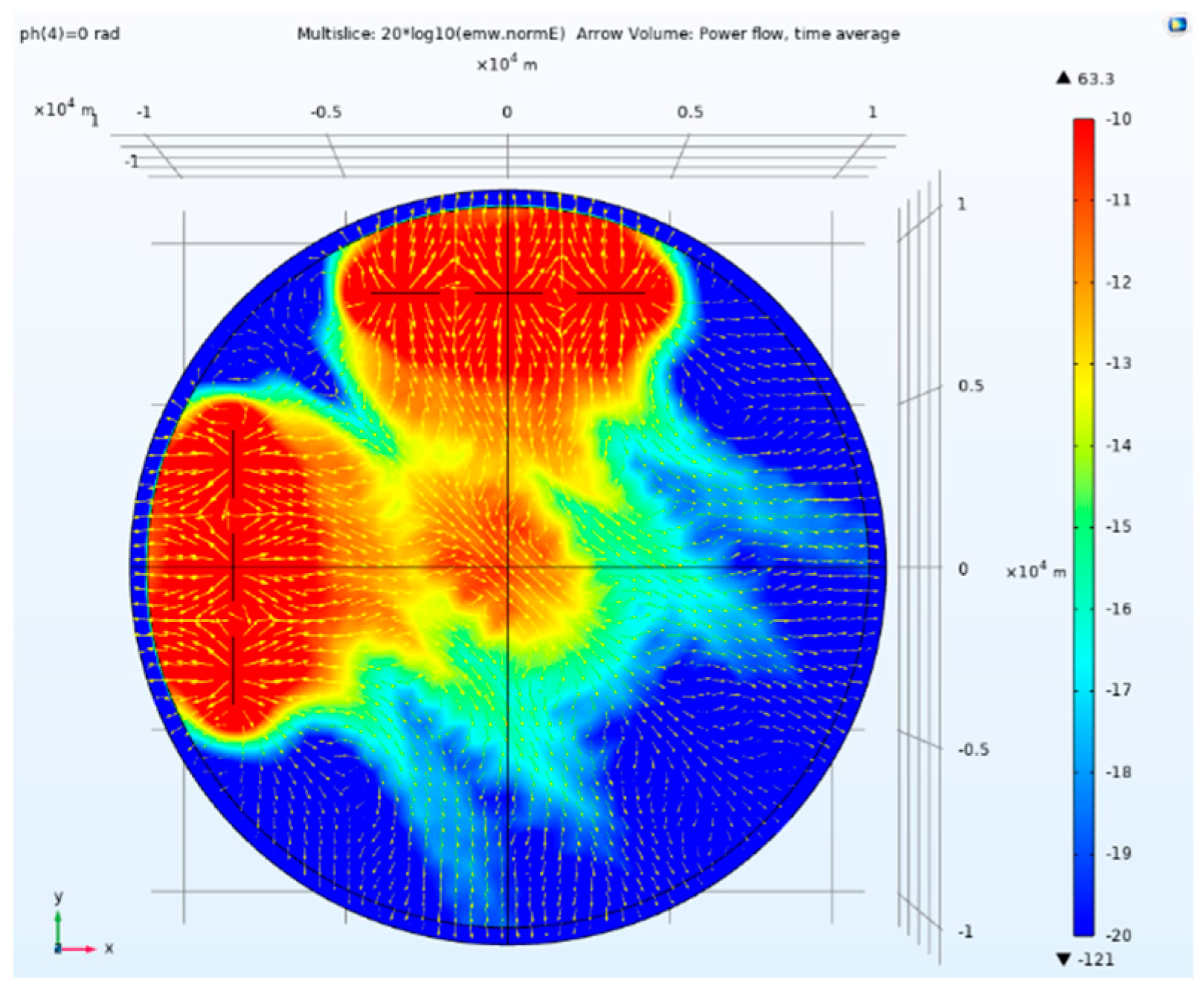
Figure 14.
Side view of electric field amplitude and direction of tensor CSAMT based on L-type array artificial field source under Taylor weighted excitation.
Figure 14.
Side view of electric field amplitude and direction of tensor CSAMT based on L-type array artificial field source under Taylor weighted excitation.
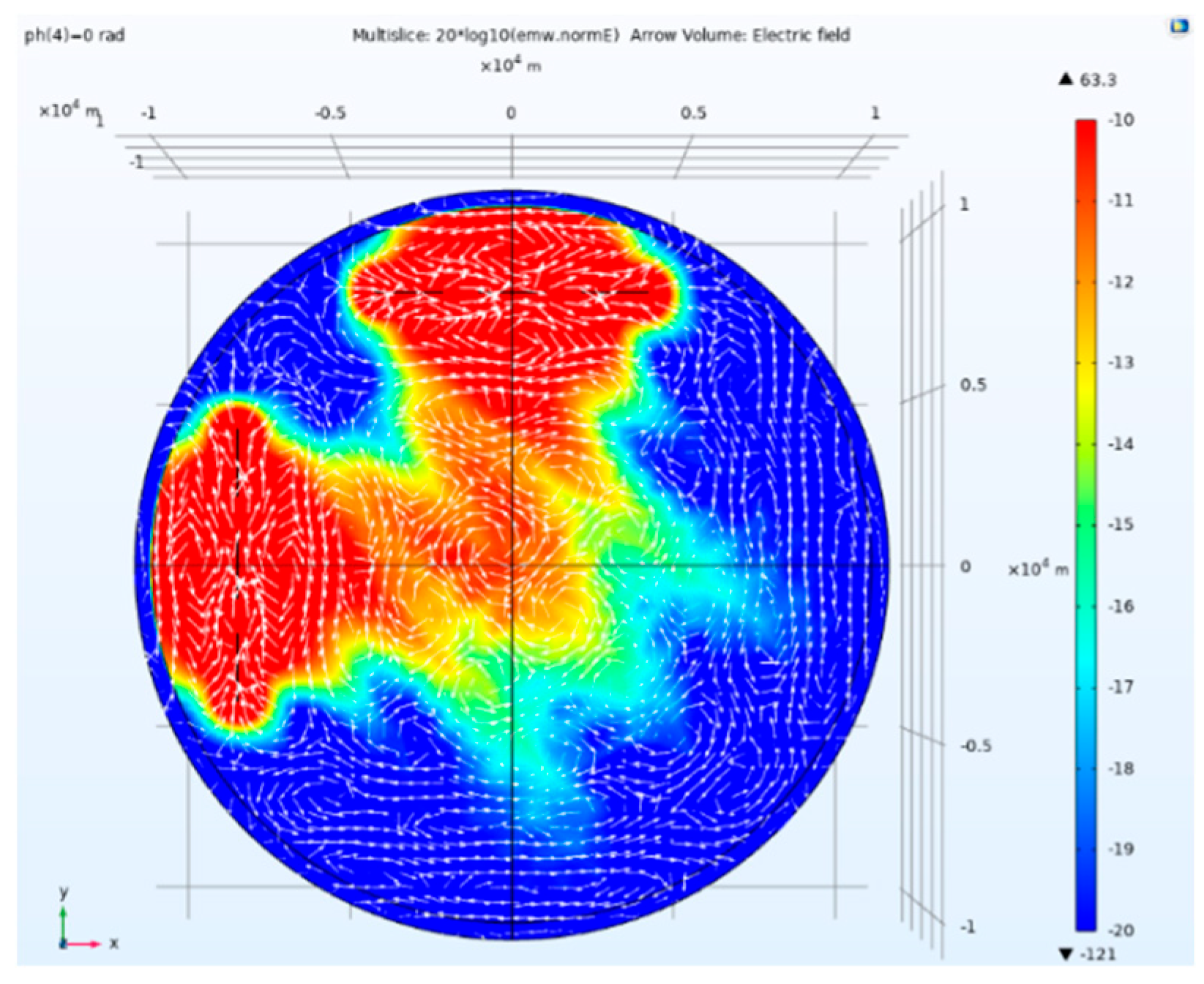
Figure 15.
Side view of magnetic field amplitude and direction of tensor CSAMT based on L-type array artificial field source under Taylor weighted excitation.
Figure 15.
Side view of magnetic field amplitude and direction of tensor CSAMT based on L-type array artificial field source under Taylor weighted excitation.
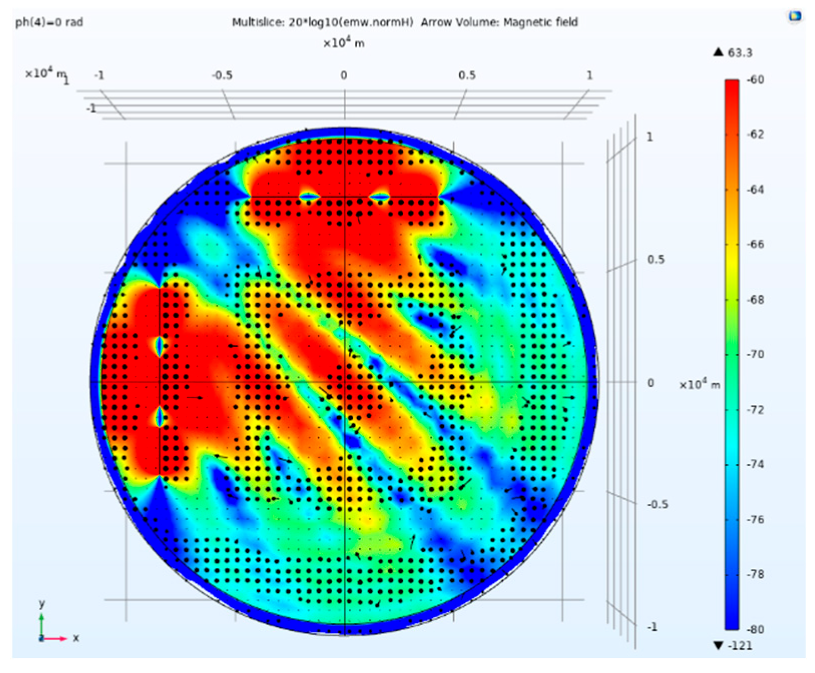
Figure 17.
Side view of electric field amplitude and direction of tensor CSAMT based on L-type array artificial field source under Taylor weighted excitation and 0.69813rad phase difference.
Figure 17.
Side view of electric field amplitude and direction of tensor CSAMT based on L-type array artificial field source under Taylor weighted excitation and 0.69813rad phase difference.
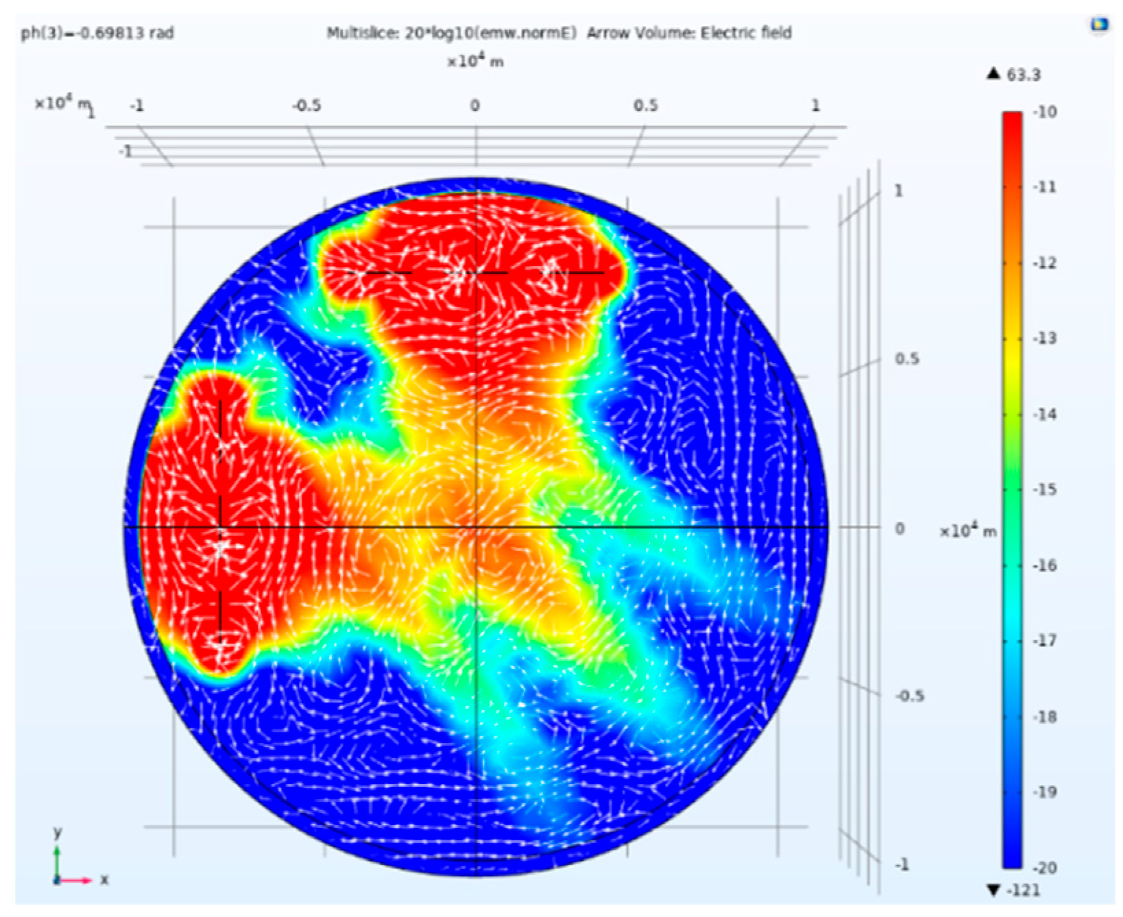
Figure 18.
Side view of electric field amplitude and direction of tensor CSAMT based on L-type array artificial field source under Taylor weighted excitation and 1.3963rad phase difference.
Figure 18.
Side view of electric field amplitude and direction of tensor CSAMT based on L-type array artificial field source under Taylor weighted excitation and 1.3963rad phase difference.
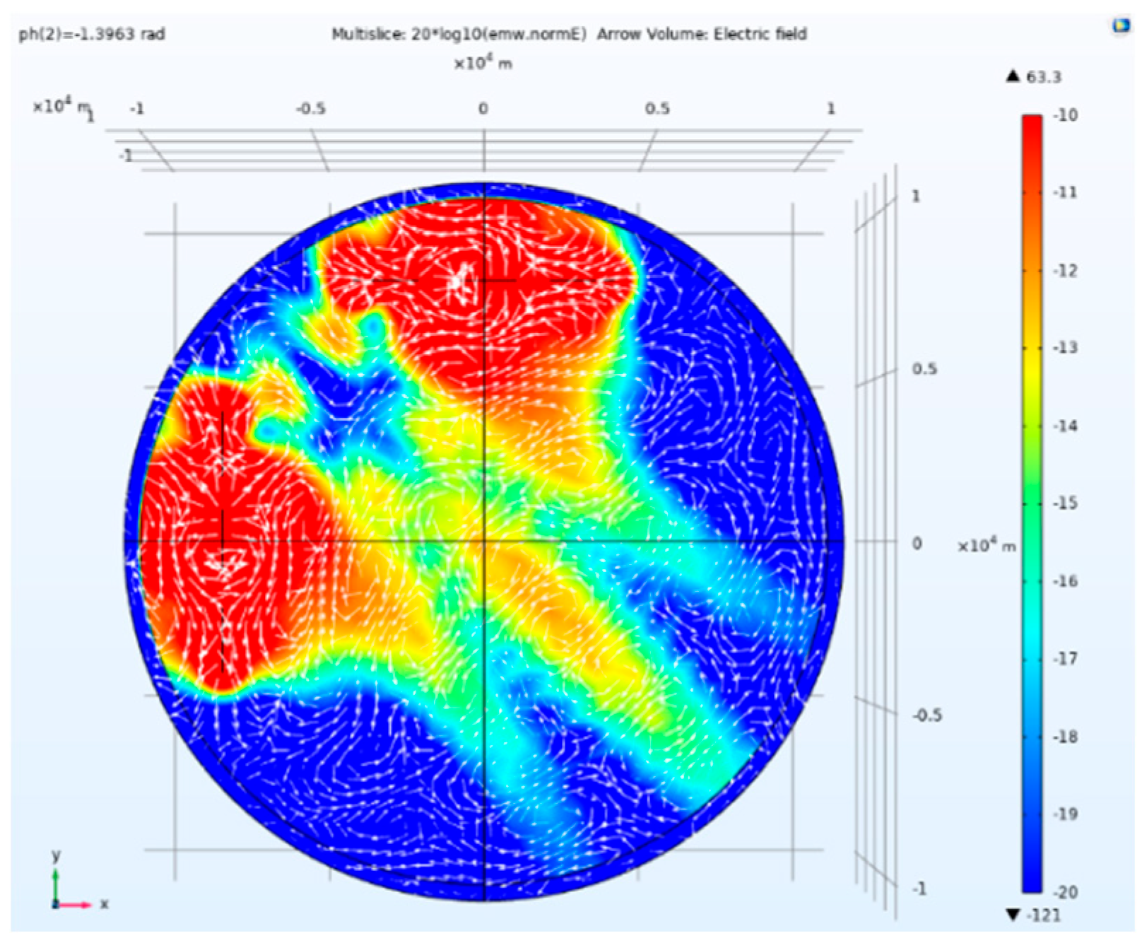
Figure 19.
Side view of electric field amplitude and direction of tensor CSAMT based on L-type array artificial field source under Taylor weighted excitation and 2.0944rad phase difference.
Figure 19.
Side view of electric field amplitude and direction of tensor CSAMT based on L-type array artificial field source under Taylor weighted excitation and 2.0944rad phase difference.
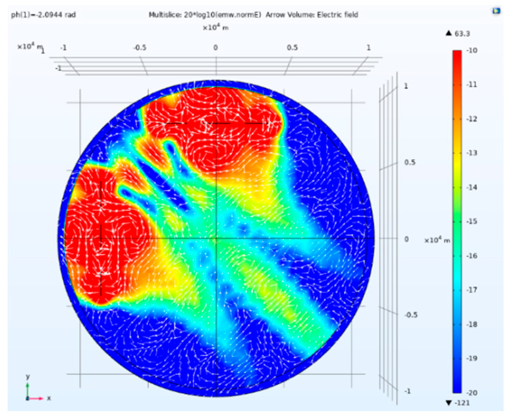
Figure 20.
Side view of magnetic field amplitude and direction of tensor CSAMT based on L-type array artificial field source under Taylor weighted excitation and 0.69813rad phase difference.
Figure 20.
Side view of magnetic field amplitude and direction of tensor CSAMT based on L-type array artificial field source under Taylor weighted excitation and 0.69813rad phase difference.
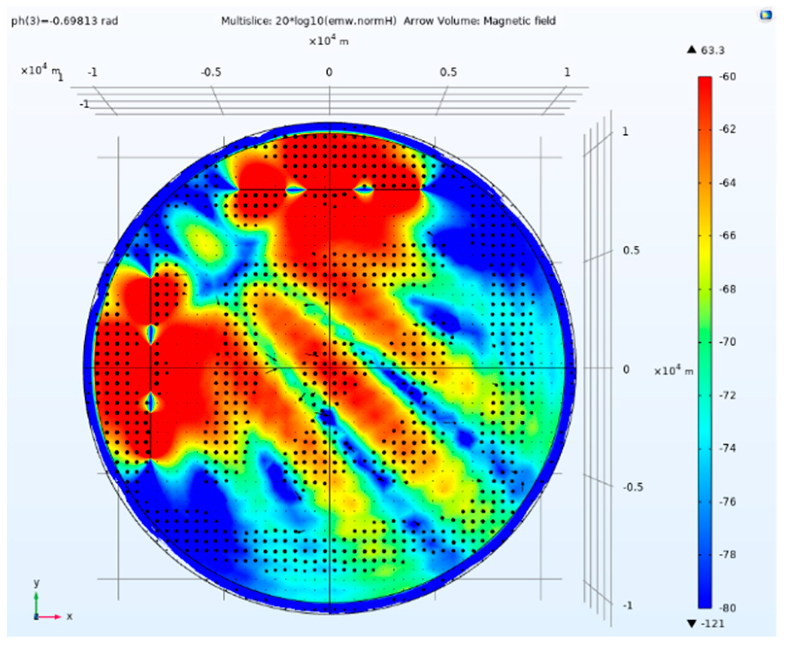
Figure 21.
Side view of magnetic field amplitude and direction of tensor CSAMT based on L-type array artificial field source under Taylor weighted excitation and 1.3963rad phase difference.
Figure 21.
Side view of magnetic field amplitude and direction of tensor CSAMT based on L-type array artificial field source under Taylor weighted excitation and 1.3963rad phase difference.
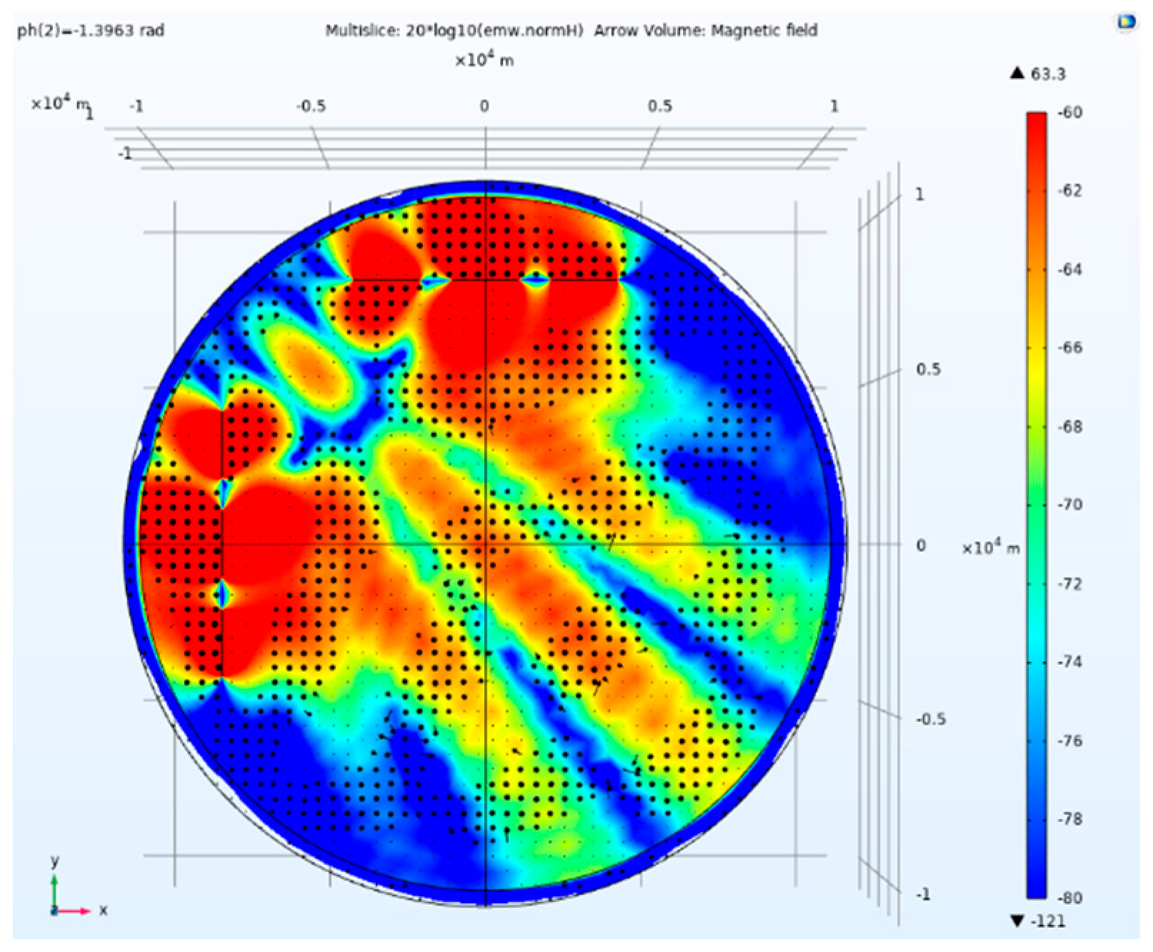
Figure 22.
Side view of magnetic field amplitude and direction of tensor CSAMT based on L-type array artificial field source under Taylor weighted excitation and 2.0944rad phase difference.
Figure 22.
Side view of magnetic field amplitude and direction of tensor CSAMT based on L-type array artificial field source under Taylor weighted excitation and 2.0944rad phase difference.
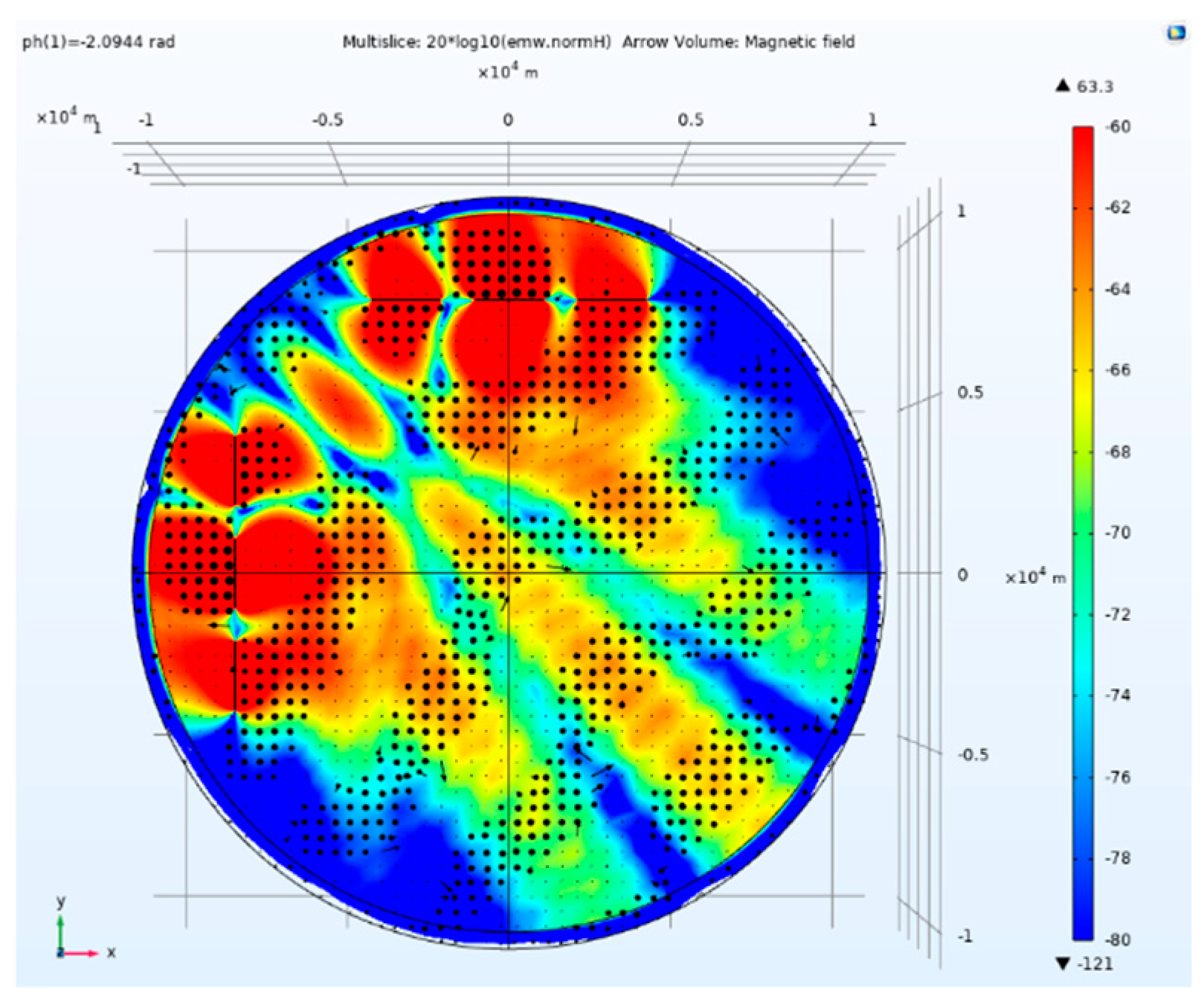
Figure 23.
Side view of electric field amplitude and Poynting vector direction of tensor CSAMT based on L-type array artificial field source under Taylor weighted excitation and 0.69813rad phase difference.
Figure 23.
Side view of electric field amplitude and Poynting vector direction of tensor CSAMT based on L-type array artificial field source under Taylor weighted excitation and 0.69813rad phase difference.
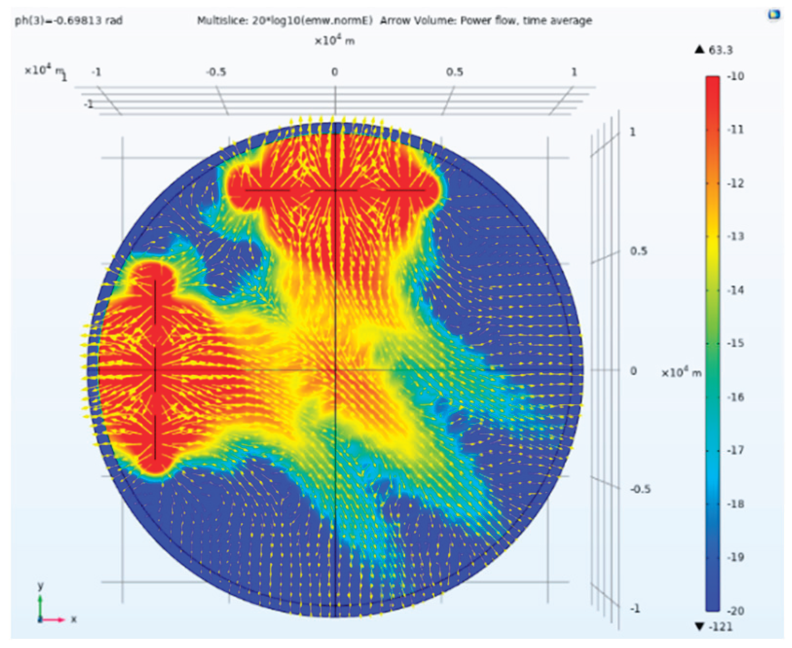
Figure 24.
Side view of electric field amplitude and Poynting vector direction of tensor CSAMT based on L-type array artificial field source under Taylor weighted excitation and 0.69813rad phase difference and 1.3963rad phase difference.
Figure 24.
Side view of electric field amplitude and Poynting vector direction of tensor CSAMT based on L-type array artificial field source under Taylor weighted excitation and 0.69813rad phase difference and 1.3963rad phase difference.
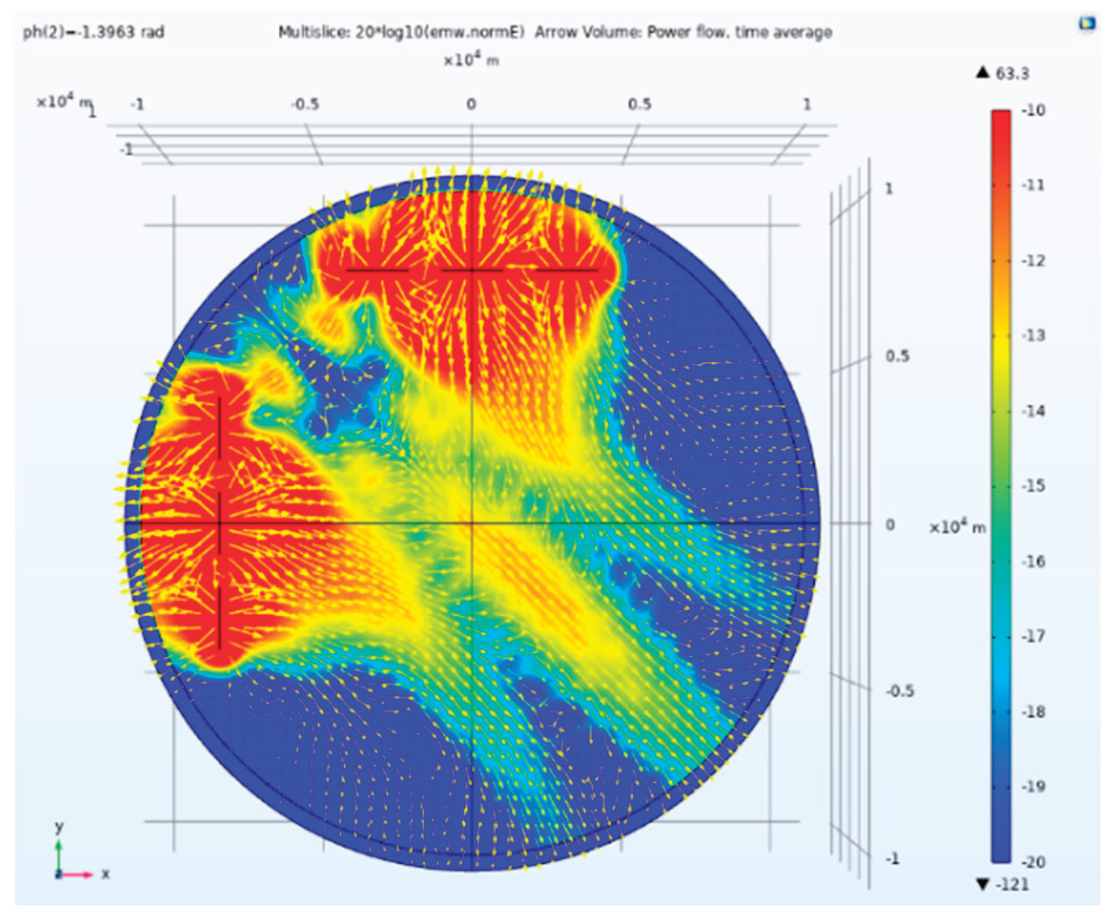
Figure 25.
Side view of electric field amplitude and Poynting vector direction of tensor CSAMT based on L-type array artificial field source under Taylor weighted excitation and 0.69813rad phase difference and 2.0944rad phase difference.
Figure 25.
Side view of electric field amplitude and Poynting vector direction of tensor CSAMT based on L-type array artificial field source under Taylor weighted excitation and 0.69813rad phase difference and 2.0944rad phase difference.
Figure 26.
Electric field amplitudes comparison of traditional tensor CSAMT, equal scale excitation and Taylor weighted based on the separation tensor CSAMT of L-type array artificial field sources.
Figure 26.
Electric field amplitudes comparison of traditional tensor CSAMT, equal scale excitation and Taylor weighted based on the separation tensor CSAMT of L-type array artificial field sources.
Figure 27.
Electric field amplitudes comparison of Taylor weighted based on the separation tensor CSAMT of L-type array artificial field sources under different phases.
Figure 27.
Electric field amplitudes comparison of Taylor weighted based on the separation tensor CSAMT of L-type array artificial field sources under different phases.
Figure 28.
Traditional separated tensor CSAMT.
Figure 29.
Electric field amplitude in x and y directions of traditional measuring point.
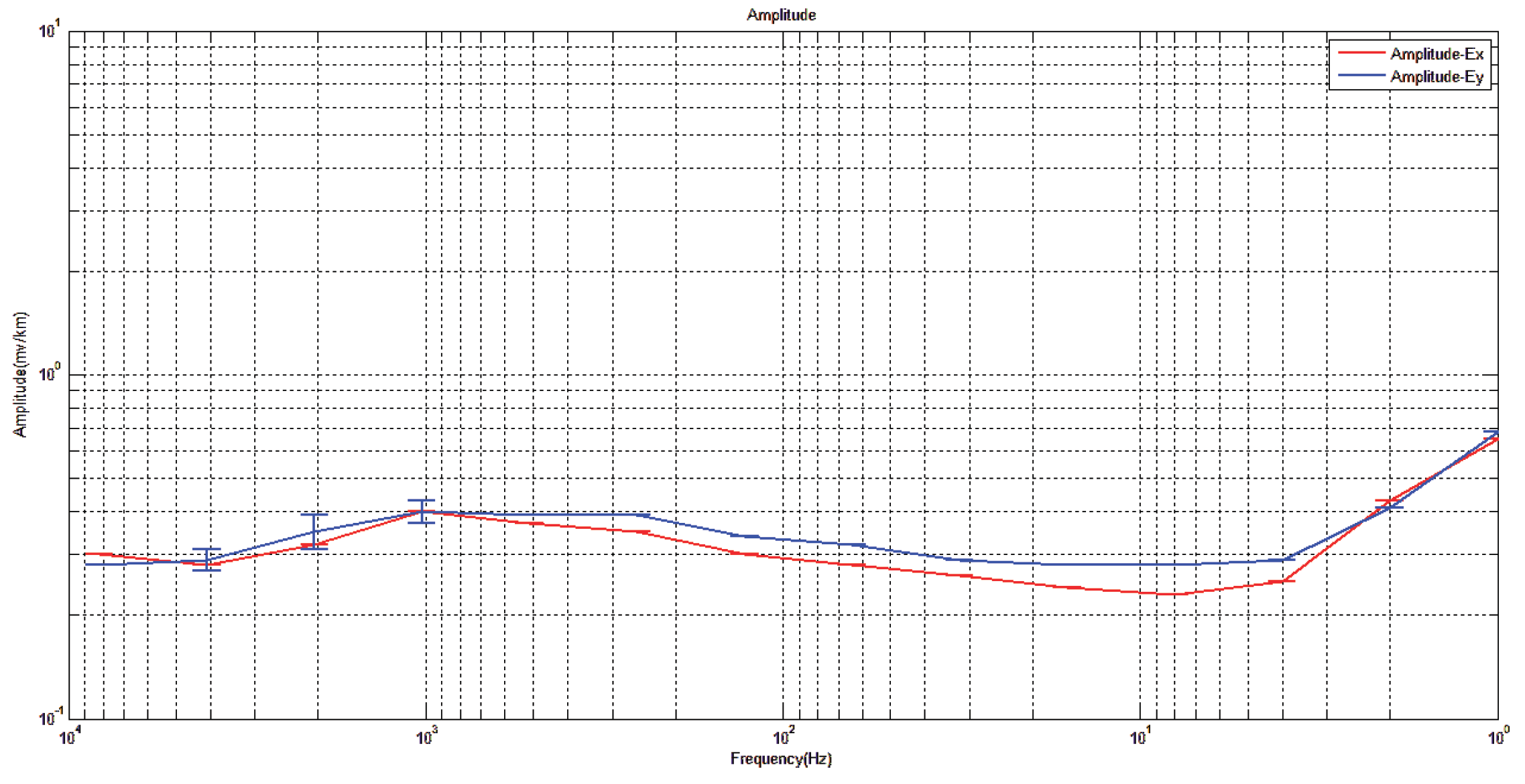
Figure 30.
Electric field amplitude in x and y directions of measuring point 1 for comparison.
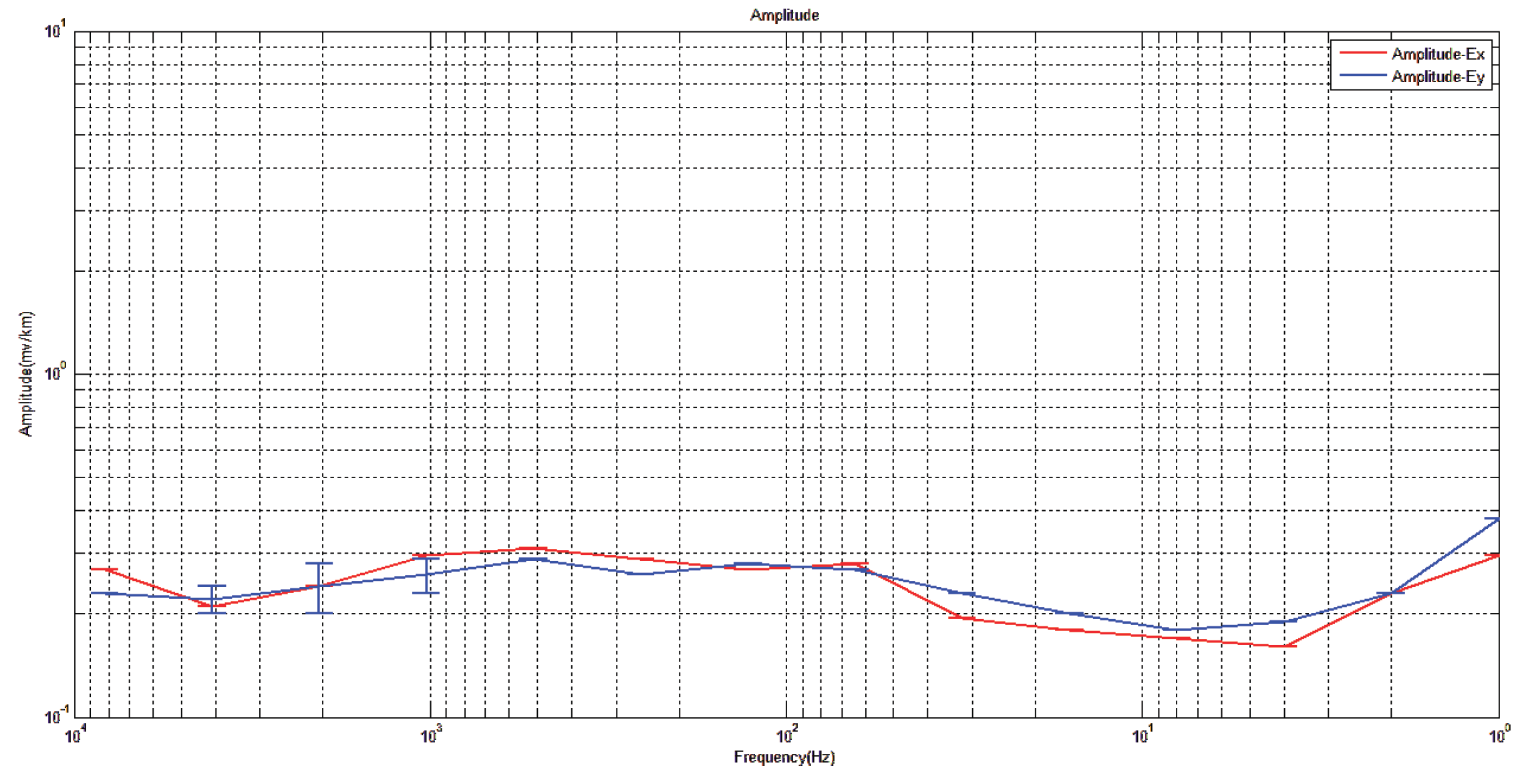
Figure 31.
Electric field amplitude in x and y directions of measuring point 2 for comparison.
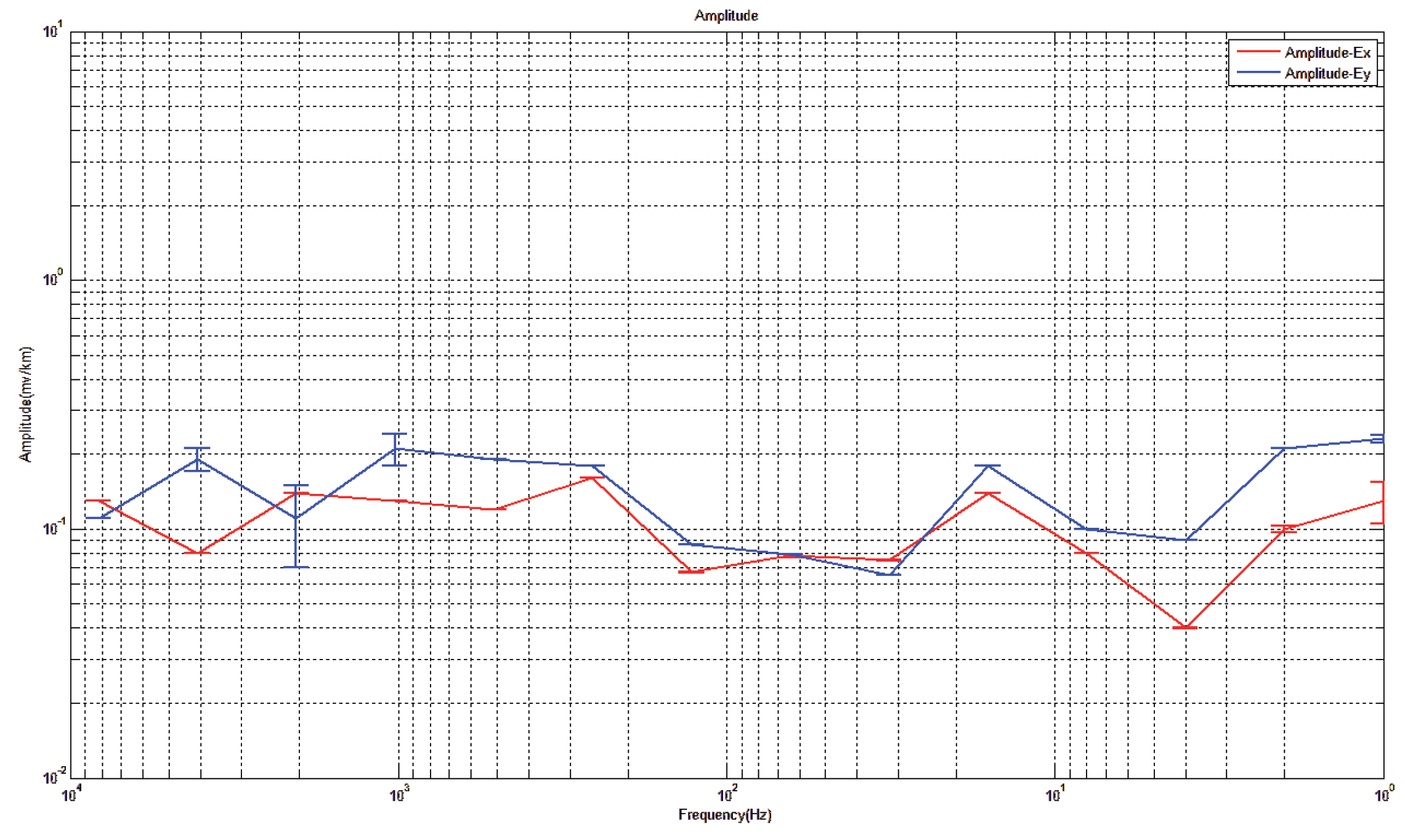
Figure 32.
Tensor CSAMT based on L-type array artificial field source.
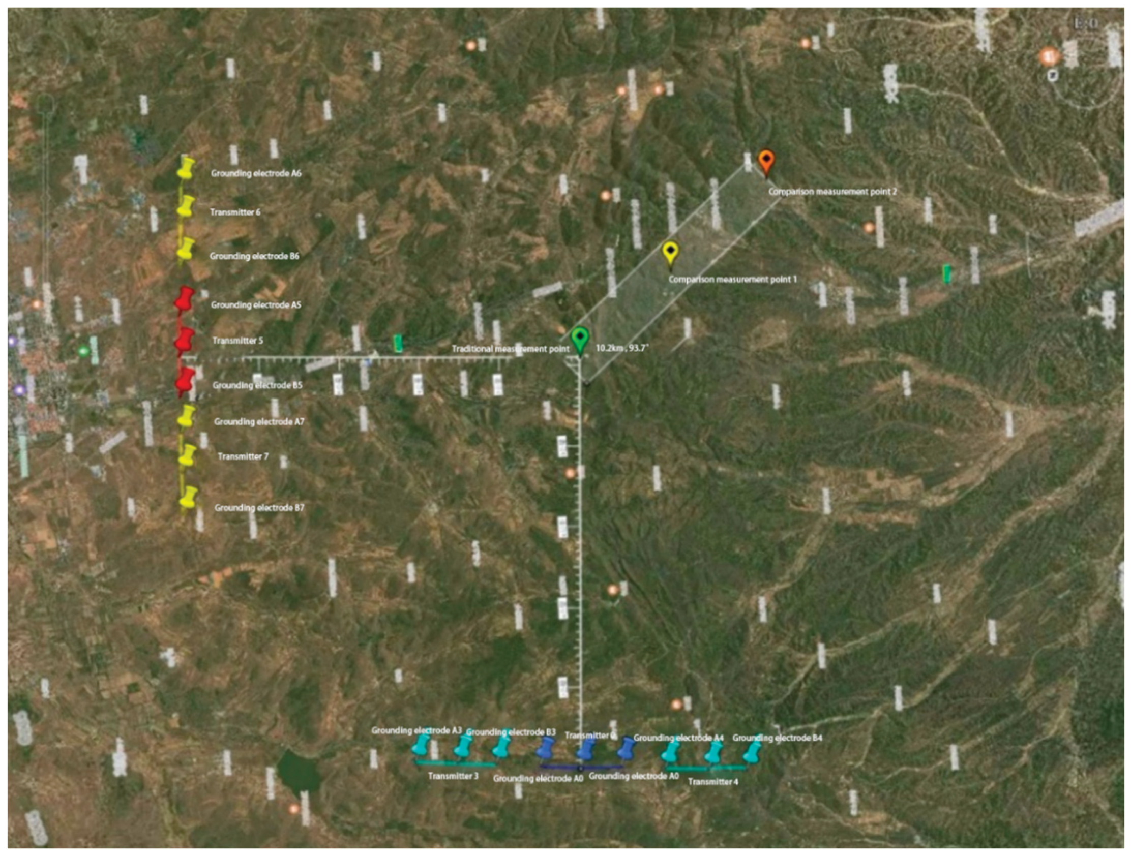
Figure 33.
Electric field amplitude in x and y directions of traditional measuring point (after pattern synthesis).
Figure 33.
Electric field amplitude in x and y directions of traditional measuring point (after pattern synthesis).
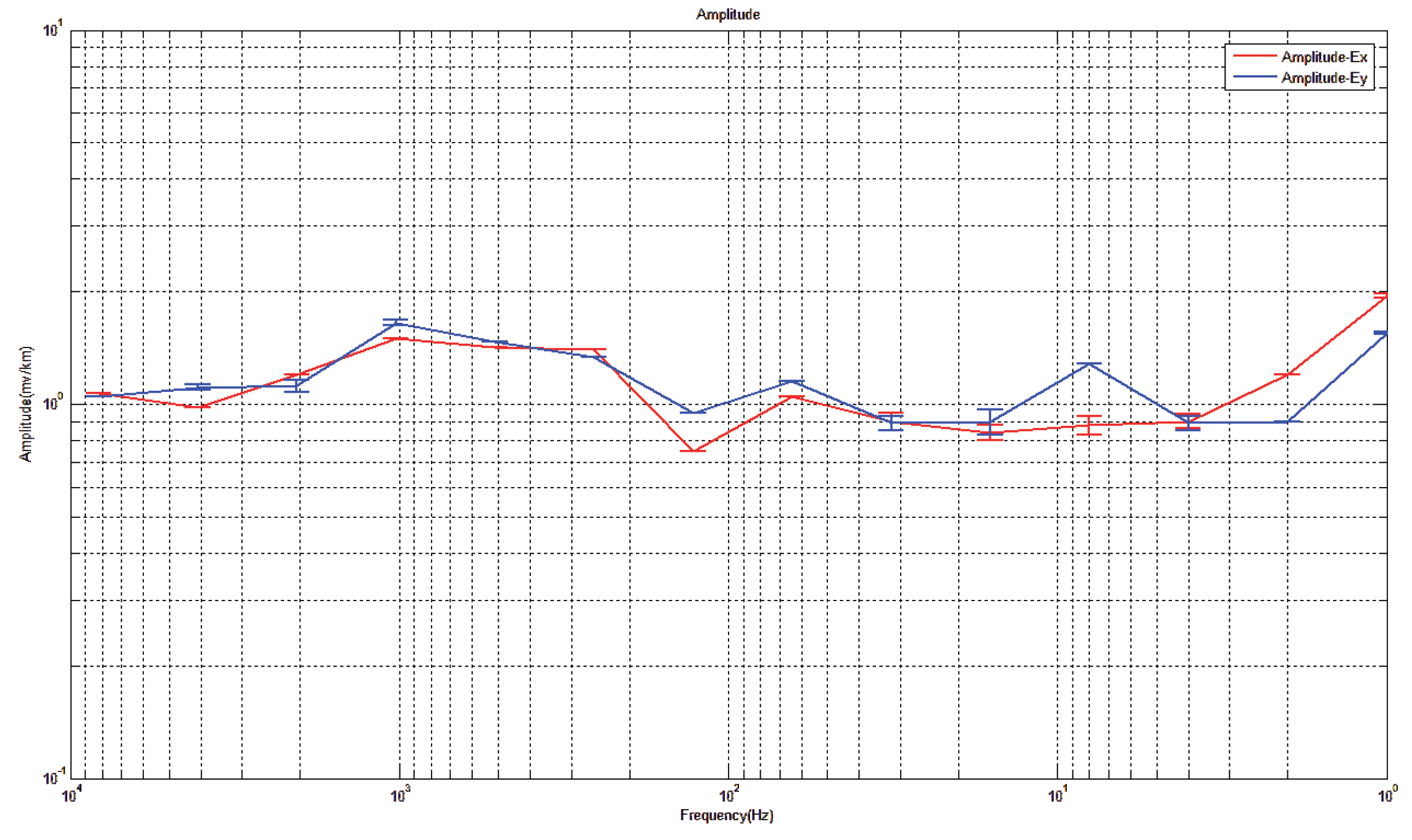
Figure 34.
Electric field amplitude in x and y directions of measuring point 1 for comparison (after pattern synthesis).
Figure 34.
Electric field amplitude in x and y directions of measuring point 1 for comparison (after pattern synthesis).
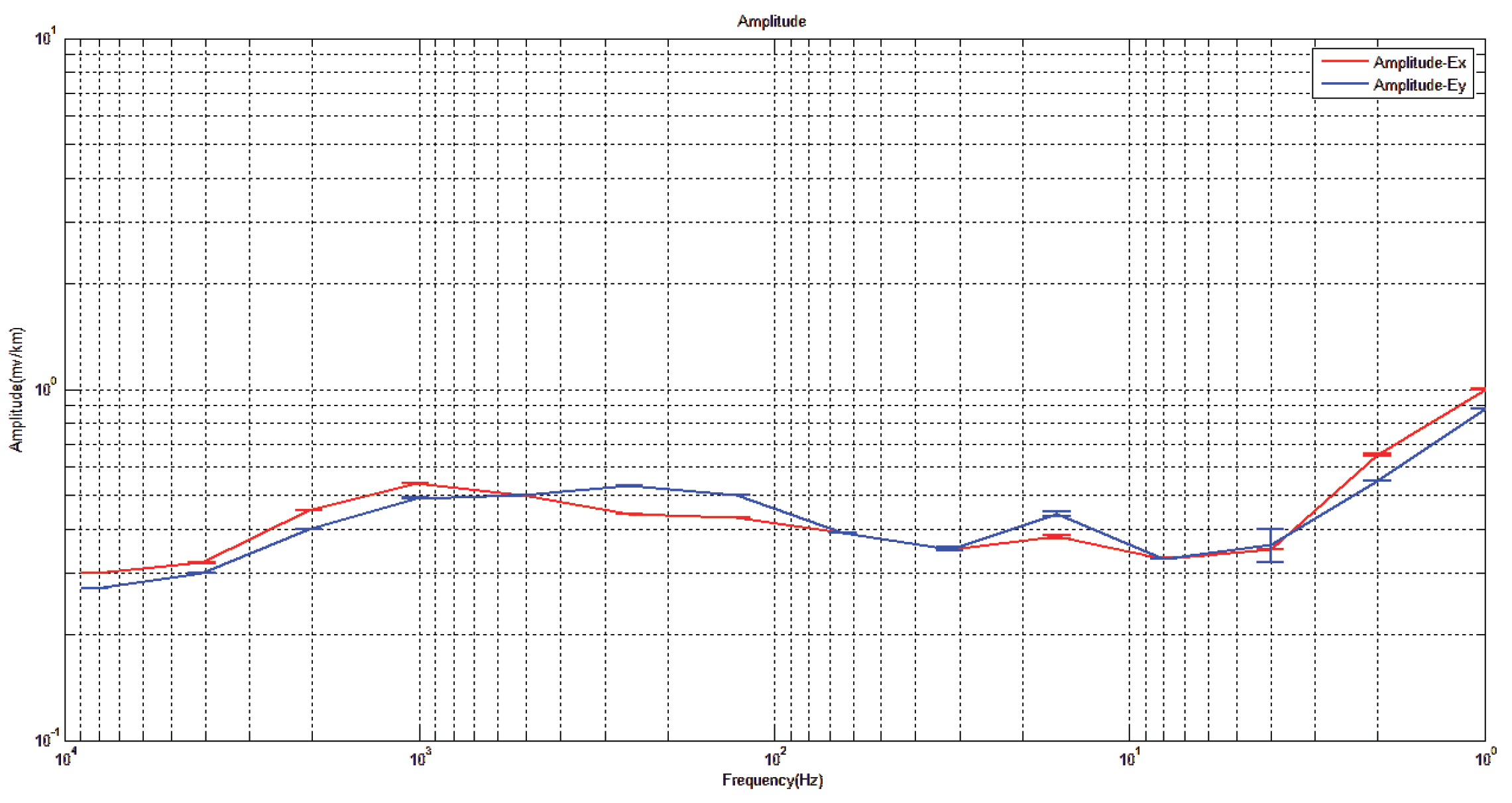
Figure 35.
Electric field amplitude in x and y directions of measuring point 2 for comparison (after pattern synthesis).
Figure 35.
Electric field amplitude in x and y directions of measuring point 2 for comparison (after pattern synthesis).
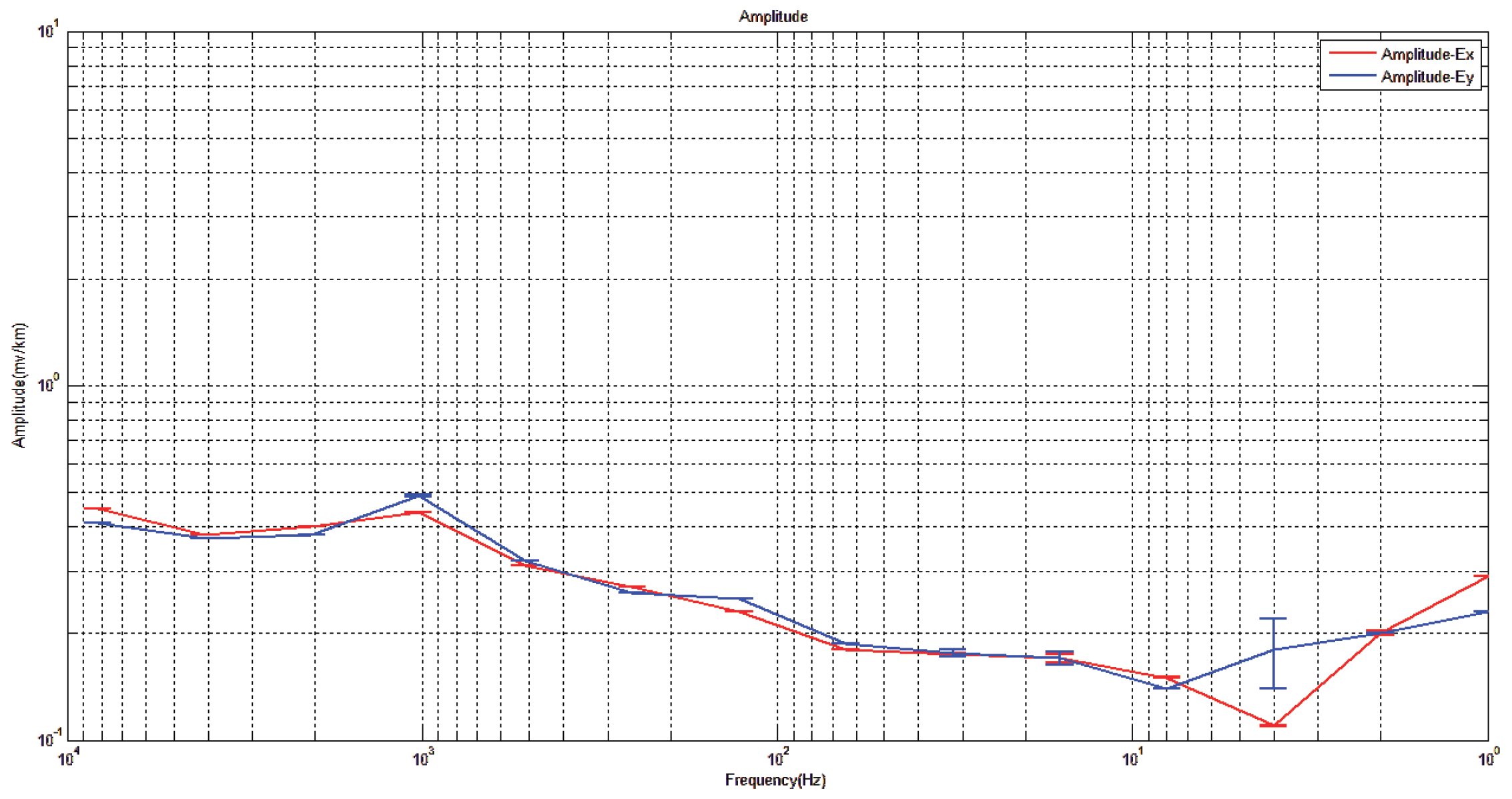
Figure 36.
Electric field amplitude in x and y direction of measuring point 1 for comparison (after adaptive beamforming).
Figure 36.
Electric field amplitude in x and y direction of measuring point 1 for comparison (after adaptive beamforming).
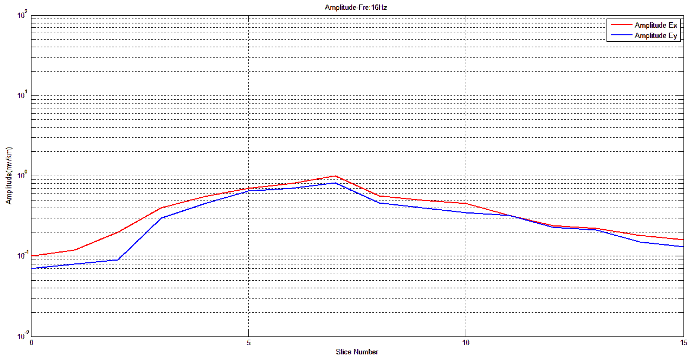
Figure 37.
Electric field amplitude in x and y direction of measuring point 2 for comparison (after adaptive beamforming).
Figure 37.
Electric field amplitude in x and y direction of measuring point 2 for comparison (after adaptive beamforming).
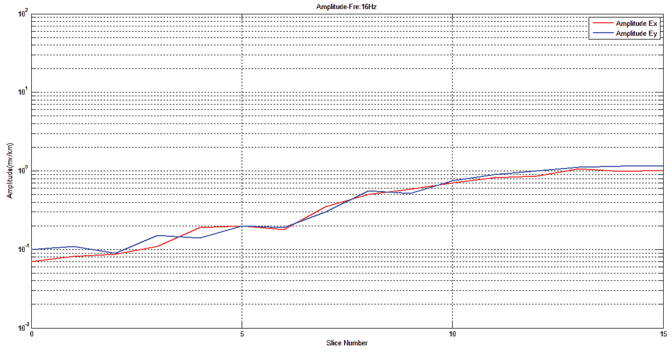

Table 1.
Arithmetic Pd for the different lumped ports, identified by their lumped port name.
| Arithmetic Phase Difference | Coaxial Resonator Linear Array Lumped Port |
| 0 [rad] | Port1 |
| ph range(-0.69813, 0.69813, -2.0944 [rad]) | Port2 |
| 2*ph [rad] | Port3 |
Table 2.
Electric field amplitudes(mV/km) comparison of traditional tensor CSAMT, equal scale excitation and Taylor weighted based on the separation tensor CSAMT of L-type array artificial field sources.
Table 2.
Electric field amplitudes(mV/km) comparison of traditional tensor CSAMT, equal scale excitation and Taylor weighted based on the separation tensor CSAMT of L-type array artificial field sources.
| (0, 0, 0) | (1000, -1000, 0) | (4000, -4000, 0) | (6000, -6000, 0) | |
| Traditional tensor | 0.44965 | 0.42756 | 0.19111 | 0.07511 |
| Equal incentive | 1.17781 | 1.11731 | 0.75391 | 0.54028 |
| Taylor Series | 1.38158 | 1.24552 | 0.93365 | 0.49438 |
Table 3.
Electric field amplitudes(mV/km) comparison of Taylor weighted based on the separation tensor CSAMT of L-type array artificial field sources under different phases.
Table 3.
Electric field amplitudes(mV/km) comparison of Taylor weighted based on the separation tensor CSAMT of L-type array artificial field sources under different phases.
| (0, 0, 0) | (1000, -1000, 0) | (4000, -4000, 0) | (6000, -6000, 0) | |
| 0rad | 1.38158 | 1.24552 | 0.93365 | 0.49438 |
| 0.69813rad | 1.24177 | 1.33122 | 1.03575 | 0.68539 |
| 1.3963rad | 1.18064 | 1.14057 | 1.23365 | 0.75419 |
| 2.0944rad | 1.08377 | 1.02522 | 1.12376 | 1.15455 |
Disclaimer/Publisher’s Note: The statements, opinions and data contained in all publications are solely those of the individual author(s) and contributor(s) and not of MDPI and/or the editor(s). MDPI and/or the editor(s) disclaim responsibility for any injury to people or property resulting from any ideas, methods, instructions or products referred to in the content. |
© 2025 by the authors. Licensee MDPI, Basel, Switzerland. This article is an open access article distributed under the terms and conditions of the Creative Commons Attribution (CC BY) license (http://creativecommons.org/licenses/by/4.0/).
Copyright: This open access article is published under a Creative Commons CC BY 4.0 license, which permit the free download, distribution, and reuse, provided that the author and preprint are cited in any reuse.


